Introduction to Analytical Mechanics
690 likes | 1.25k Vues
Introduction to Analytical Mechanics. Lagrange’s Equations. Siamak G. Faal 1/1 07/29/2016. Rigid body dynamics. Dynamic equations: Provide a relation between forces and system accelerations Explain rigid body motion and trajectories. Image sources (left to right):

Introduction to Analytical Mechanics
E N D
Presentation Transcript
Introduction to Analytical Mechanics Lagrange’s Equations Siamak G. Faal 1/1 07/29/2016
Rigid body dynamics Dynamic equations: • Provide a relation between forces and system accelerations • Explain rigid body motion and trajectories Image sources (left to right): https://www.etsy.com/listing/96803935/funnel-shaped-spinning-top-natural-wood https://spaceflightnow.com/2016/06/30/juno-switched-to-autopilot-mode-for-jupiter-final-approach/ https://upload.wikimedia.org/wikipedia/commons/d/d8/NASA_Mars_Rover.jpg http://www.popularmechanics.com/cars/a14665/why-car-suspensions-are-better-than-ever/
Kinematics vs Kinetics Image sources (left to right): https://www.youtube.com/watch?v=PAHjo4DXOjc http://www.timelinecoverbanner.com/facebook-covers/billiard.jpg
Dynamic Forces and Reactions Dynamic analysis are essential to determine reaction forces that are cussed by dynamic forces (e.g. Accelerations) Image sources (left to right): http://r.hswstatic.com/w_404/gif/worlds-greatest-roller-coasters-149508746.jpg http://www.murraymitchell.com/wp-content/uploads/2011/04/red_aircraft_performing_aerobatics.jpg
Differential Equations of Motion provide a set of differential equations which allow modeling, simulation and control of dynamic mechanical systems Why humanoid robots do not walk or act like humans !?
Notations Throughout this presentation: • Vectors are noted with overlines: • The first derivative with respect to time: • The second derivative with respect to time:
Time Derivative of a Vector Time derivative of a vector in rotating coordinate frame is: Angular velocity of the frame Relative rate of change of the vector
Newtonian Dynamics Newton laws of motion: • The velocity of a particle can be changed by the application of a force • The resultant force is proportional to the acceleration of particle with the factor of mass • The forces acting on a body result from an interaction with another body. The action and reaction forces have the same magnitude, the same line of action but opposite directions
Newtonian Equations of Motion For each rigid body: Linear momentum of the center of mass: Time derivative of the angular momentum of the object about point A Vector from arbitrary point A to G (center of mass) Acceleration of the arbitrary point A
Newtonian Equations of Motion A simplified form of the equations are achieved by considering the following assumptions: • Mass of the object is constant • Moment equations are calculated at the center of mass
Energy Kinetic energy of a rigid body: Potential energy of an object with mass located at altitude due to gravity: Potential energy stored in an spring with stiffness :
Degrees of Freedom The number of independent parameters that define system configuration In planar motion A free object has DOF In 3D space A free object has DOF 3 6
Mechanical Joints Revolute joint Adds 5 constraints Relative DOF: 1 Planar joint Adds 3 constraints Relative DOF: 3 Spherical joint Adds 3 constraints Relative DOF: 3 Prismatic joint Adds 5 constraints Relative DOF: 1 Cylindrical joint Adds 4 constraints Relative DOF: 2
Generalized Coordinates A set of geometrical parameters which uniquely defines the position / configuration of the system The minimum number of generalized coordinates that required to specify the position of the system is equal to the number of DOF of the system (unconstrained or independent coordinates) Generalized coordinates do not form a unique set! Generalized coordinates are commonly notes with
Generalized Coordinates Q) What can be a set of generalized coordinates for a simple rod in on a plane. A)
Generalized Coordinates Q) Can you think about any other generalized coordinates set for the same system? A)
Generalized Coordinates Q) How about another one? A) This is an ambiguous set of coordinates!
Generalized Coordinates Here we have more coordinates than the digress of freedom of the system, Thus the coordinates can not have any arbitrary value and they need to satisfy two constrain equations: Q) Let’s do one more A)
Constraints Any generalized coordinate which can not have any arbitrary value is a constrained coordinate Relation between constrained generalized coordinates is called constraint equation : Number of constraint equations Number of degrees of freedom Number of constrained generalized coordinates
Virtual Displacement In a virtual movement, the generalized coordinates of the system are considered to be incremented by infinitesimal amount from the values they have at an arbitrary instant, with time held constant. Path due to force 2 Path due to force 1
Virtual Displacement Example: Generalized coordinate: Q) What are the virtual displacements of pin F and virtual rotation of bar EF resulting from B A C D E F
Virtual Displacement Solution: A B C D E F
Virtual Work When a particle is given a virtual displacement , the forces acting on the particle do virtual work Since is infinitesimal, is infinitesimal as well Because the change is virtual, time is held constant at an arbitrary value The virtual work done by constraint or internal forces is zero!
Generalized Forces Generalized force
Joseph-Louis Lagrange 25 January 1736 – 10 April 1813, Italian Enlightenment Era mathematician and astronomer. Lagrangemade significant contributions to the fields of analysis, number theory, and both classical and celestial mechanics. Lagrange’s Equations
Lagrange’s Equations of Motion Alternative (common) form:
Lagrange’s Equations of Motion • Directly provides the differential equations of motion without any need for solving a system of equations. • Provides a much easier method to solve multi-body systems • It is very systematic and can be used to automatically generate differential equations of motion for different systems (As long as the derivatives are computed correctly)
Example 1 Find differential equations of motion for the following system using both Newtonian mechanics and Lagrange’s equations
Example 1 Newtonian approach: Spring force is equal to: Assume Newton’s second law for x-axis: Since the only force applied to the system is the spring force: So the differential equation of motion for the system is: Free-body diagram:
Example 1 Lagrangian approach: The kinetic energy of the system is: The potential energy of the system is: Since there is no force acting on the system, the generalized force is zero: Lagrangian of the system is: Thus, the differential equation of motion is: Calculations:
Example 2 Find differential equations of motion for the following system using both Newtonian mechanics and Lagrange’s equations
Example 2 Newtonian approach: Spring force is equal to: Assume Newton’s second law for x-axis: The summation of forces along x axis is: So the differential equation of motion for the system is: Free-body diagram:
Example 2 Lagrangian approach: The kinetic energy of the system is: The potential energy of the system is: The generalized force acting on the system is: Lagrangian of the system is: Thus, the differential equation of motion is: Calculations:
Example 3 Find differential equations of motion for the following system using both Newtonian mechanics and Lagrange’s equations
Example 3 Newtonian approach: Moment of inertia of a rod: Moment equation around point O gives us: Free-body diagram:
Example 3 Lagrangian approach: Center of mass position in terms of generalized coordinates The kinetic energy of the system is: The potential energy of the system is:
Example 3 Lagrangian approach (cont.): The generalized force is Lagrangian of the system is: Thus, the differential equation of motion is: Calculations:
References [1] Ginsberg, Jerry H. Advanced engineering dynamics. Cambridge University Press, 1998. [2] Greenwood, Donald T. Advanced dynamics. Cambridge University Press, 2006.