Download

1 / 45
450 likes | 592 Vues
This lecture by Dr. James Demmel and Dr. Kathy Yelick from the University of California, Berkeley, covers the classical N-body problem, which simulates the evolution of systems influenced by gravitational and electrostatic forces. It explores applications in astrophysics, particle physics, and molecular dynamics. Key topics include particle methods, the Barnes-Hut algorithm for efficient computation, and the use of adaptive structures like quad trees and octrees to optimize force calculations among large bodies. Understanding these algorithms enhances simulations in cosmology and related fields.

E N D
Cosmology ApplicationsN-Body Simulations Credits: Lecture Slides of Dr. James Demmel, Dr. Kathy Yelick, University of California, Berkeley CS267, Yelick
Introduction Classical N-body problem simulates the evolution of a system of N bodies The force exerted on each body arises due to its interaction with all the other bodies in the system
Motivation • Particle methods are used for a variety of applications • Astrophysics • The particles are stars or galaxies • The force is gravity • Particle physics • The particles are ions, electrons, etc. • The force is due to Coulomb’s Law • Molecular dynamics • The particles are atoms or • The forces is electrostatic • Vortex methods in fluid dynamics • Particles are blobs of fluid CS267, Yelick
Particle Simulation t = 0 while t < t_final for i = 1 to n … n = number of particles compute f(i) = force on particle i for i = 1 to n move particle i under force f(i) for time dt … using F=ma compute interesting properties of particles (energy, etc.) t = t + dt end while • N-Body force (gravity or electrostatics) requires all-to-all interactions • f(i) = Sk!=i f(i,k) … f(i,k) = force on i from k • Obvious algorithm costs O(N2), but we can do better... CS267, Yelick
Reducing the Number of Particles in the Sum • Consider computing force on earth due to all celestial bodies • Look at night sky, # terms in force sum >= number of visible stars • One “star” is really the Andromeda galaxy, which is billions of stars • A lot of work if we compute this per star … • OK to approximate all stars in Andromeda by a single point at its center of mass (CM) with same total mass • D = size of box containing Andromeda , r = distance of CM to Earth • Require that D/r be “small enough” D r Earth D Andromeda x r = distance to center of mass x = location of center of mass CS267, Yelick
x Using points at CM Recursively • From Andromeda’s point of view, Milky Way is also a point mass • Within Andromeda, picture repeats itself • As long as D1/r1 is small enough, stars inside smaller box can be replaced by their CM to compute the force on Vulcan • Boxes nest in boxes recursively Replacing clusters by their Centers of Mass Recursively D r Earth D Andromeda Vulcan r1 D1 D1 CS267, Yelick
Quad Trees • Data structure to subdivide the plane • Nodes can contain coordinates of center of box, side length • Eventually also coordinates of CM, total mass, etc. • In a complete quad tree, each nonleaf node has 4 children CS267, Yelick
Oct Trees • Similar Data Structure to subdivide 3D space • Analogous to 2D Quad tree--each cube is divided into 8 sub-cubes Two Levels of an OctTree CS267, Yelick
Using Quad Trees and Oct Trees • All our algorithms begin by constructing a tree to hold all the particles • Interesting cases have non-uniform particle distribution • In a complete tree (full at lowest level), most nodes would be empty, a waste of space and time • Adaptive Quad (Oct) Tree only subdivides space where particles are located • More compact and efficient computationally, but harder to program CS267, Yelick
Example of an Adaptive Quad Tree Adaptive quad tree where no space contains more than 1 particle Child nodes enumerated counterclockwise from SW corner Empty ones excluded CS267, Yelick
Barnes-Hut Algorithm • High Level Algorithm (in 2D, for simplicity) 1) Build the QuadTree using QuadTree.build … already described, cost = O( N log N) 2) For each node = subsquare in the QuadTree, compute the CM and total mass (TM) of all the particles it contains … “post order traversal” of QuadTree, cost = O(N log N) 3) For each particle, traverse the QuadTree to compute the force on it, using the CM and TM of “distant” subsquares … core of algorithm … cost depends on accuracy desired but still O(N log N) CS267, Yelick
Step 3: Compute Force on Each Particle • For each node, can approximate force on particles outside the node due to particles inside node by using the node’s CM and TM • This will be accurate enough if the node if “far enough away” from the particle • Need criterion to decide if a node is far enough from a particle • D = side length of node • r = distance from particle to CM of node • q = user supplied error tolerance < 1 • Use CM and TM to approximate force of node on box if D/r < q D r Earth D Andromeda x r = distance to center of mass x = location of center of mass CS267, Yelick
Computing Force on a Particle Due to a Node • Use example of Gravity (1/r2) • Given node n and particle k, satisfying D/r < q • Let (xk, yk, zk) be coordinates of k, m its mass • Let (xCM, yCM, zCM) be coordinates of CM • r = ( (xk - xCM)2 + (yk - yCM)2 + (zk - zCM)2 )1/2 • G = gravitational constant • Force on k ~ G * m * TM * xCM – xk yCM – yk zCM – zk ----------- ---------- ---------- r3 r3 r3 CS267, Yelick
Parallelization Three phases in a single time-step: tree construction, tree traversal (or force computation), and particle advance Each of these must be performed in parallel; a tree cannot be stored at a single processor due to memory limitations Step 1: Tree construction - Processors cooperate to construct partial image of the entire tree in each processor
Step 1: Tree Construction Initially, the particles are distributed to processors such that all particles corresponding to a subtree of hierarchical domain decomposition are assigned to a single processor Each processor can independently construct its tree The nodes representing the processor domains at the coarsest level (branch nodes) are communicated to all processors using all-to-all Using these branch nodes, the processor reconstructs the top parts of the tree independently There is some amount of replication of the tree across processors since top nodes in the tree are repeatedly accessed
Step 2: Force Computation • To compute the force on a particle (belonging to processor A) by a node (belonging to processor B), processors need to communicate if the particle and the node belong to different processors • Two methods: • Children of nodes of another processor (proc B) are brought to the processor containing the particle (proc A) for which the force has to be computed • Also called as data-shipping paradigm • Follows owner-computes rule
Step 2: Force computation • Method 2: Alternatively, the owning processor (proc A) can ship the particle coordinates to the other processor (proc B) containing the subtree • Proc B then computes the contribution of the entire subtree on particle • Sends the computed potential back to proc A • Function-shipping paradigm: computation (or function) is shipped to the processor holding the data • Communication volume is less when compared to data-shipping
Step 2: Force Computation • In function-shipping, it is desirable to send many particle coordinates together to amortize start-up latency: • A processor keeps storing its particle coordinates to bins maintained for each of the other processor • Once a bin reaches a capacity, it is sent to the corresponding processor • Processors must periodically process remote work requests
Load Balancing In applications like astrophysical simulations, high energy physics etc., the particle distributions across the domain can be highly irregular; hence tree may be very imbalanced Method 1: Static partitioning, static assignment (SPSA) Partition the domain into r subdomains, r >> p processors Assign r/p subdomains to each processor Some measure of load balance if r is sufficiently large
Load Balancing Method 2: Static Partitioning, Dynamic Assignment (SPDA) Partitioning the domain into r subdomains or clusters as before Follow dynamic load balancing at each step based on the loads of the subdomains E.g.: Morton Ordering
Morton Ordering Morton ordering is an ordering/numbering of the subdomains: the bits of the row and column are interleaved and the subdomains/clusters are labeled by Morton number The Morton ordered subdomains are located nearby each other mostly; when this ordered subdomains is partitioned across processors, nearby interacting particles/nodes are mapped to a single processor, thus optimizing communication
Load Balancing using Morton Ordering • The ordered subdomains are stored in a sorted list • After an iteration, a processor computes the load in each of its clusters; the load is entered into sorted list • The load at each processor is added to form a global sum • The global sum is divided by the number of processors, to form equal load • The list is traversed and divided such that the loads in each division (processor) is approximately equal
Load Balancing using Morton Ordering • Each processor compares the load in current iteration with the desired load in the next iteration • If current load < desired load, clusters/subdomains are imported from next processor in Morton ordering • If not, excess load clusters exported from the end of current list to next processor • Done at end of each iteration
Load Balancing Method 3: Dynamic Partitioning, Dynamic Assignment (DPDA) Allow clusters/subdomains of varying sizes Each node in the tree maintains the number of particles it interacted with After force computation, this summed along the tree; the value of load at each node now stores the number of interactions with all nodes rooted at the subtree; the root node contains the total number of interactions, W, in the system The load is partitioned into W/p; the corresponding load boundaries are 0, W/p, 2W/p,…,(p-1)W/p The load balancing problem now becomes locating one of these points in the tree
Load Balancing Each processor traverses its local tree in an in-order fashion and locates all load boundaries in its subdomain All particles lying in the tree between load boundaries iW/p and (i+1)W/p are collected in a bin for processor i and communicated to processor i
Load Balancing: Costzones DPDA scheme is also referred to as the costzones scheme The costs of computations are partitioned The costs are predicted based on the interactions in the previous time step In classical N-body problems, the distribution of particles changes very slowly across consecutive time steps Since a particle’s cost depends on the distribution of particles, a particle’s cost in one time-step is a good estimate of its cost in the next time step A good estimate of the particle’s cost is simply the number of interactions required to compute the net force on that particle
Load Balancing: Costzones Partition the tree rather than partition the space In the costzones scheme, the tree is laid in a 2D plane The cost of every particle is stored with the particle Internal cell holds the sum of the costs of all particles that are contained within it The total cost in the domain is divided among processors so that every processor has a contiguous, equal range or zone of costs (hence the name costzones) E.g.: a total cost of 1000 would be split among 10 processors so that the zone comprising costs 1-100 is assigned to the first processor, zone 101-200 to the second, and so on.
Load Balancing: Costzones The costzone a particle belongs to is determined by the total cost up to that particle in an inorder traversal of the tree Processors descend the tree in parallel, picking up the particles that belong to their costzone Internal nodes are assigned to processors that own most of their children – to preserve locality of access to internal cells
Fast Multipole Method (FMM) In this method, a cell is considered far enough away or “well-separated” from another cell b if its separation from b is >= the length of b Cells A and C are well-separated from each other Cell D is well-separated from C But C is not well-separated from D
FMM: Differences from B-H • B-H computes only particle-cell or particle-particle interactions; FMM computes cell-cell interactions; This makes force computations phase in FMM O(n) • In FMM, well-separatedness depends only on cell sizes and distances, while in B-H, it depends on user-parameter theta • The FMM approximates a cell not by its mass, but by a higher-order series expansion of particle properties about the geometric center of the cell; The expansion is called multipole expansion; the number of terms in the expansion determines accuracy • But more complicated to program
FMM: Force Computations Efficiency of FMM is improved by allowing a larger maximum number of particles per leaf cell in the tree; typically 40 particles per leaf cell For efficient force calculation, every cell C divides the rest of the computational domain into a set of lists of cells, each list containing cells that bear a certain spatial relationship to C
FMM: Force Computations First step is to construct these lists for all cells Interactions of every cell are computed with ONLY the cells in its lists Thus no cell C ever computes interactions with cells that are well-separated from its parent (e.g., blank cells in the figure)
FMM Parallelization • The parallelization steps (tree construction, force computations by function shipping) and load balancing schemes are similar to Barnes-Hut • The primary differences: • The basic units of partitioning are cells, which, unlike particles in B-H • Partitioning like ORB schemes becomes more complicated (next slide) • Force-computation work associated not only with the leaf cells of the tree, but with internal cells as well • Costzones scheme should also consider the cost of the internal nodes while partitioning; Internal nodes/cells holds the sum of all cells within it plus its own cost
FMM: ORB Scheme Since the unit of parallelization is a cell, when a space is bisected in ORB, several cells are likely to straddle the bisecting line (unlike particles in B-H) Hence ORB is done in 2 phases In the 1st phase, cells are modeled as points at their centers; a cell that straddles the bisecting line is given to whichever subspace its center happens to be in But this can result in load imbalances since an entire set of straddling cells can be given to one or the other side of the bisector
FMM: ORB Scheme Hence in the 2nd phase, a target cost for each subdomain is first calculated as half the total cost of the cells in both subdomains The border cells are visited in an order sorted by position along the bisecting axis, and assigned to one side of the bisector until that side reaches the target cost The rest of the border cells are then assigned to the other side of the bisector
References The paper "Scalable parallel formulations of the Barnes-Hut method for n-body simulations" by Grama, Kumar and Sameh. In Supercomputing 1994. The paper "Load balancing and data locality in adaptive hierarchical N-body methods: Barnes-Hut, Fast Multipole, and Dardiosity" by Singh, Holt, Totsuka, Gupta and Hennessey. In Journal of Parallel and Distributed Computing, 1994 CS267, Yelick