Download
1 / 81
810 likes | 843 Vues
Explore the fundamentals of digital images, from representations to properties. Learn about image digitization, color images, camera functions, and more. Dive into the essentials of spatial, radiometric, spectral, and temporal resolutions, as well as image quality and noise. Gain insights into image segmentation, noise parameters estimation, and histogram computation.

E N D
Ch. 2 – The image, its representation, type, and properties 2.1. Image Representations and Concepts 2.2. Image Digitization 2.3. Digital Image Properties 2.4. Color Images 2.5. Cameras
○ Function 2.1. Image Representations and Concepts • Continuous – A, B: continuous • Discrete – A: discrete, B: continuous • Digital – A, B: discrete ○ Scene g(x,y,z): a 3-D continuous function Digital imagef(x,y): a 2-D digital function Origin ○ Pixel: picture element Gray level: pixel value
○ Image Formation Pin-hole camera 2-2
○ Perspective Projection Pin-hole model
2 mm ○ Drawbacks of pinhole camera: (i) Big pinhole - Averaging rays blurs image Small pinhole - Diffraction effect blurs image 1 mm 0.35 mm 0.15 mm 0.07 mm (ii)Images are relatively dark Solution : *Pinholes Lenses Lenses: gather light sharp focus
2.2. Image Digitization Camera Sensor array Image array
Types of resolutions: • Spatial (space) • Radiometric (intensity) • Spectral (color) • Temporal (time) 2-6
2.2.2. Radiometric Resolution (Quantization) False contours
Non-uniform resolution -- to reduce storage while preserve as much information as possible Non-uniform * Spatial resolution (sampling): Sharp region – fine, dense Smooth area – coarse, sparse * Radiometric resolution (quantization): Busy area – fine, dense Inactive region – coarse, sparse * Spectral resolution (quantization): * Time resolution (sampling):
Non-Uniform Sampling 64 by 64 128 by 128 Uniform sampling Non-uniform sampling
Adaptive sampling 128 by 128 64 by 64 Adaptive mesh Input image Gradient image Spring model Sampled image Adapted mesh
2.3. Digital Image Properties ○Adjacency 8-neighbors 4-neighbors ○ Metric Properties (i) Distances Euclidean City-block Chess-board
Quasi-Euclidean (ii) Distance Transform (Chamfering)
○Geometrical Properties (i) Crack edges: each pixel has 4 crack edges e.g., (ii) Inner, outer borders (iii) Convex, concave (vi) Convex hull: the smallest convex region containing the input region
○Topological properties (i) Rubber Sheet Transform (RST):preserves the contiguity of object parts and the number of holes in regions (no cut and joint). e.g., Imagine a rubber balloon with an object painted on it (ii) Euler-Poincare Characteristic: Euler number (#regions - #holes) is invariant under RST (iii) Topological components:
2.3.2. Histograms Probability distribution Histogram
2.3.3. Entropy Information theory -- amount of information Physical system -- measure of disorder Confidence theory -- amount of uncertainty Image -- degree of redundancy
2.3.4. Visual Perception (i) Perceptual Grouping (Organization)
(ii) Simultaneous Contrast (iii) Overshoot and Undershoot (iv) Subjective Objects Mack band pattern 2-22
Are the lines parallel or not? (v) Optical Illusion and Visual Phenomena The human brain tricks us whenever it can! 2-23
Coil or circle? 2-24
It doesn‘t move! 2-26
It doesn‘t move too! 2-27
It doesn‘t move too! 2-28
Concentrate on the cross in the middle, after a while you will notice that this moving purple dot will turn green! Look at the cross a bit longer and you‘ll notice that all dots except the green one will disappear. 2-29
2.3.5. Image Quality Image degradationresults from: (i) noise n, (ii) degradation process H , such as error, distortion, and blurring Degradation model: Additive Multiplicative where g(x,y): input image, f(x,y): degraded image H: degradation process, n(x,y): noise
Degradation processes H Additivity: Homogeneity: Linearity: Position (or space) invariance:
Image: Degraded image: If H is linear, If H is homogeneous, : impulse response of H Let : point spread function (PSF) Then,
If H is position invariant, Then, Simplified degradation model: In frequency domain,
2.3.6. Noise in Images -- Originating from image acquisition, digitization, or transmission Additive: Multiplicative: e.g., Physical processes e.g., Television raster, film material ○ White noise:the noise whose Fourier spectrum is constant FT 2-34
○ Random noise: Objectives: i) examine the performance of a developed algorithm ii) help to remove noise from an image (i) Salt-and-pepper (impulse) noise 2-35
(iii) Rayleigh noise (iv) Erlang (gamma) noise
(v) Exponential noise (vi) Gaussian noise 2-39
Method 1: 2-41
Method 2: 若p為均勻分佈,則F-1(p)為常態分佈
Error FunctionErf(x) Definition: By Taylor expansion:
Method 3: 2-44
Image segmentation (i) manually or (ii) automatically ◎ Estimation of noise parameters Gaussian Rayleigh Uniform
Steps: 1. Segment the image 2. Choose a large uniform image region 3. Compute its histogram 4. Compute the mean and variance of the histogram 5. Determine the probability distribution from the shape of the histogram 6. Estimate the parameters of the probability distribution of the histogram
Example: Rayleigh noise: From From 2-47
Measures of Image Quality 1.Signal-to-Noise Ratio (SNR) (logarithmic scale) 2. Peak Signal-to-Noise Ratio (PSNR) where I: input image, K: output image
2.4. Color Images 2.4.1. Physics of Color -- The world is colorless. Human color perception is carried out by the nervous system, which interprets differently to distinct electromagnetic wavelengths. -- Electromagnetic spectrum 2-49