Download

1 / 44
440 likes | 572 Vues
CS 795 – Computer Security Architectures. Using Markov Process in the Analysis of Intrusion Tolerant Systems. Quyen L. Nguyen. References. Sheldon M. Ross. “Introduction to Probability Models”, Academic Press.

E N D
CS 795 – Computer Security Architectures Using Markov Process in the Analysis of Intrusion Tolerant Systems Quyen L. Nguyen
References • Sheldon M. Ross. “Introduction to Probability Models”, Academic Press. • KishorShridharbhaiTrivedi. “Probability and Statistics with Reliability, Queuing, and Computer Science Applications, 2nd Edition”. Wiley-Interscience, 2001. • Bharat B. Madan, KaterinaGoseva-Popstojanova, KalyanaramanVaidyanathan, and Kishor S. Trivedi. “A Method for Modeling and Quantifying the Security Attributes of Intrusion Tolerant Systems”. Performance Evaluation 56 (2004), 167-186. • KhinMi MiAung, Kiejin Park, and JongSou Park. “A Model of ITS Using Cold Standby Cluster”. ICADL 2005, LNCS 3815, pp. 1-10, 2005. • Alex Hai Wang, Su Yan and peng Liu. “A Semi-Markov Survivability Evaluation Model for Intrusion Tolerant Database Systems”. 2010 International Conference on Availability, Reliability and Security. • Quyen Nguyen and ArunSood. “Quantitative Approach to Tuning of a Time-Based Intrusion-Tolerant System Architecture”. WRAITS 2009, Lisbon, Portugal. Note: State Diagrams and matrix snapshots in subsequent slides are taken from [3], [4] and [5].
Outline • Markov Chain • Semi-Markov Process (SMP) • Analysis Model of ITS • Mean Time to Security Failure (MTTSF) • Availability • SCIT • Cluster • ITDB
Stochastic Process • Given that it rains today, will it rain or shine tomorrow? • Given that it is sunny today, will it rain or shine tomorrow?
Markov Process • State space: {rainy, sunny} • Parameter space: X1, X2, … • Markov property: next state depends only on current state • pij= p(Xn+1 = j | Xn= i, Xn-1 = in-1, …, X0 = i0) = p(Xn+1 = j | Xn= i) • Transition Probability Matrix: • P = [pij] with ∑jpij= 1 for every i • Markov Chain: finite state space • Discrete-time, Continuous-time
Steady-state Probabilities • Stationary Process: transition probability independent of n • p(Xn+1 = j | Xn= i) = p(Xn = j | Xn-1 = i) • Chapman-Kolmogorov for n-step transition matrix • P(n) = Pn • Pnconverges to steady state values, as n --> ∞ • Solution of system (1) of equations: • x.P = x • Σi xi= 1
Semi-Markov Process • Time spent in a state i is a random variable with mean µ1 • If amount of time in each state is 1, then SMP is a Markov. • Embedded DTMCwith steady-state probabilities πi • Time proportion in state i: • Pi = (πi * µi) / ∑j (πj * µj) (2) • Steps to solve an SMP: • Solve steady-probabilities of DTMC using system (1) • Use (2)
Modeling ITS • Modeling steps: • Identify states • Identify transitions • Assign transition probabilities
DTMC Transition Probability Matrix [3] • p1 = 1 - pa • p2 = 1 – pm – pu • p3 = 1 – ps - pg
Calculating Availability [3] • A = 1 – (PFS + PF + PUC) • Transition Diagram and formula depend on attack scenario and metric to compute. • Example: DoS attack, remove unused states MC and FS: • A = 1 – (PF + PUC)
Availability: Numerical Examples [3] • A is decreasing function of Pa and increasing function of hG.
Absorbing and Transient States • if pij = 0 for i ≠ j, then i is an absorbing state. • Example: complete system failure state. • Arranging Transition Probability, with Q containing transitions between transient states only.
Visit Times • k-step transition probability matrix Pk • ∑Qk = I + Q1 + Q2 + … converges to (I – Q)-1 = M = [mij] • (I – Q)-1 = M ↔ M(I – Q) = I ↔ M = I + MQ • Theorem: Let Xijbe the visit times of state j starting from state i before going to absorbing states: E[Xij]= mij • Starting from state 1, V = (V1, V2, …, Vn) can be solved by system of equations: • V = I + V.Q
Calculating MTTSF • Determine absorbing states: {UC, FS, GD, F}. • Transient states: {G, V, A, MC, TR} • Form transition matrix comprising of transient states Q. • Compute visit times Vi using the equations: • v = q + v.Q • MTTSF = v.µ
MTTSF Numerical Examples [3] • MTTSF decreases as Pa increases • MTTSF increases as hG increases.
Issues • Parameter Modeling • Probability Distribution: exponential, Weibull, etc. • Mean value Estimation
SCIT Parameters • Online window Wo: server accepts requests from the network • Grace period Wg: server stops accepting new requests and tries to fulfill outstanding requests already in its queue. • Exposure window: W = Wo + Wg. • Nonline: # redundant online nodes. • Ntotal : total nodes in the cluster. • Ntotal, W, and the cleansing-time Tcleansing are inter-related.
SCIT: State Transition Diagram with Absorbing States • Pa: probability of successful attack • Pc: probability of cleansing when in A. • F: low chance of occurrence, but still possible: • Virtual machine and/or the host machine no longer respond to the Controller. • Controller itself fails due to a hardware fault.
SCIT: MTTSF Computation • Xa and Xt are absorbing states and transient states Xa = {F} and Xt = {G, V, A} • q: probabilities that process starts at each state in Xt : q = (1,0,0), since it starts with state G. • V = (V0 V1 V2): number of visit times for each state in Xt. • h: mean sojourn times in each state • Solve system of equations: V = q + VQ • Using solutions for V, compute MTTSFscit = V.h Q
SCIT: MTTSF Expression • Pa↓ → MTTSFscit↑ • Pc↑ → MTTSFscit↑ • How to make Pa↓ and Pc↑?
SCIT: Relationship between Pa and W • Modeling malicious attack arrivals: • Assumption: non-staged attacks • (Attack arrivals) ̴ Poisson (λ) • Then, inter-arrival time Y between attacks is exponential distribution: • P(Y ≤ W) = 1 - e-λW • P(Y ≤ W) is also prob. that attacks occur in exposure window. • Then: • Pa ≤ P(Y ≤ W) • → Pa ≤ 1 - e-λW
SCIT: Relationship between Pc and W • Resident time of the attack modeled as a “service” time Z with rate μ. • Assume Z exponential distribution: P(Z > W) = e-μW • probability that the service time is greater than W is limited by the fact that the system moves out of state A due to the cleansing mode: • P(Z > W) ≤ Pc ↔ Pc ≥ e-µW • System cannot “serve” more than the arriving attacks: μ ≤ λ. • Then: e-μW≥ e-λW .
SCIT: MTTSF and W • W ↓→ (Pa ≤ 1 - e-λW) ↓ • W ↓→ (Pc ≥ e-µW) ↑ • Then: W ↓→ MTTSFscit↑ • MTTSFSCIT ≥ F(W), where F(W) is a decreasing function of W: • Significance: engineer instance of SCIT architecture by tuning W in order to increase or decrease the value of MTTSFSCIT.
SCIT Failure State • Is state F really absorbing? • Compromise of Controller is very minimal due to the one-way data. • System automatically recovers back to the G state. • Use Semi-Markov Process with embedded DTMC (Discrete-Time Markov Chain) to compute the steady-state Availability (state without security faults).
SCIT: Availability • Solve the DTMC steady-state probabilities vector y = (y0, y1, y2, y3) for all states in {G, V, A, F}: • y = y.P • Σiyi = 1.
SCIT: Availability and Exposure Window • Compute SMP stead-state probability πF for state F: • πF = y3h3/y.h, with h = (h0, h1, h2, h3) being extended to include the mean sojourn time h3 for state F. • Availability = 1 − πF • Availability monotonically decreases with Pa but increases with Pc. • Using the same line of reasoning and the assumption of Poisson attack arrival process as for MTTSFSCIT above, we can also conclude that decreasing the exposure window will increase Availability .
Rejuvenation: Single System [4] • Rejuvenation: stop software, clean internal state, service restart. • Reconfiguration: patching, anti-virus, access control (IP blocking, port blocking, session drop, content filtering), traffic control by limiting bandwidth. • Both may be needed depending on the situation.
Rejuvenation: Transition Probability [4] • Equation System: • π = π.P and Σiπi = 1. • πi, i= (H,I,J,C,F). • A = 1 – (πF + πJ + πC ) • Paper uses balance equations of probabilities leaving and entering a state.
Rejuvenation: Cluster Analysis [4] • Use SMP for modeling with State Space: Xs = • {(1,1), (I,1), (J,1), (C,1), (F,1), (0,1), (0,I), (0,J), (0,C), (F,F)} • d is the solution of DTMC equations:d.P and Σdi = 1 • Then, the prob. for SMP is given by: • A = 1 – (πF 1 + πFF ) • Deadline D of mean sojourn time (dihi). • Indicator variable Y: • Yi = 0 if dihi ≤ D and Yi= 1 if dihi > D • Survavibility S = • A – [YJ1πF 1 + YC1πC1 + Y0Jπ0J + Y0Cπ0C]
Rejuvenation: Numerical Results [4] • As prob.for (Rj,1), (Rc,1) or (0,Rj), (0,Rc) increase, availability and survivability decrease.
Rejuvenation: Numerical Results [4] • Changes of survability vs. changes in rejuvenation when attacked. • No significant difference between deadlines when prob < .4
Coping Ability: Numerical Results [4] • Survivability is maximized when primary-secondary servers detect abnormal behavior early.
ITDB: State Transition [5] • Integrity: fraction of time when all accessible data are clean • I = πG + πQ + πR • Availability: fraction of time when all clean data are accessible • A = πG + πR
ITDB: False Alarm Rate [5] • ITDB maintains I and A even at high FA rate. • Degradation of I and A as FA increases.
ITDB: Detection Rate [5] • ITDB depends on detection probability. • When Pd = 0, I and A are at low level. • When Pd increases, I and A go up. • ITDB can maintain I and A at some level at low detection rate. d
ITDB: Attack Rate [5] • Heavy attack: hG = 5. • Compare “good” and “poor” systems in terms of Pd, Pfa, hI, hQ, hR. • When attack rate increases, observe: • I and A • Q and R d
Summary • What is a Markov Process? • How to model an ITS using a Semi-Markov Process? • How to calculate MTTSF based on the model? • Application to SCIT Analysis • Rejuvenation Cluster Analysis • ITDB Analysis
Thank You! mailto:qnguyeng@gmu.edu