Cool loops, transequatorial loops and coronal waves
Cool loops, transequatorial loops and coronal waves. An MSSL compilation (Louise Harra, Sarah Matthews, Lidia van Driel-Gesztelyi) with help (Cristina Mandrini, Alphonse Sterling). Cool loops in active regions. First seen with Skylab, routinely observed by CDS

Cool loops, transequatorial loops and coronal waves
E N D
Presentation Transcript
Cool loops, transequatorial loops and coronal waves An MSSL compilation (Louise Harra, Sarah Matthews, Lidia van Driel-Gesztelyi) with help (Cristina Mandrini, Alphonse Sterling)
Cool loops in active regions • First seen with Skylab, routinely observed by CDS • Temperature range 2x10⁴ – 106 K • Both complete and partial loops are seen • Contrast generally high and behaviour is dynamic (e.g. Kjeldseth-Moe & Brekke, 1998, Harra-Murnion et al., 1999) • Conflicting reports about the relationship between hot and cool plasma • Are they cooling /structures? Heating? What is the role of e.g. siphon flows
Observations • 3 AR on the limb were studied with CDS, SXT and MDI • O v and SXT intensity revealed variability (EJECT_V3) • O v velocities show flows • MDI data was used to determine magnetic field direction • Parallel/anti-parallel flows in both legs => siphon flows • Oppositely directed flows in each leg => heating or cooling
O v with SXT contours O v with SXT contours Flare 1 ~ 18:30 Flare 2 ~ 22:30
Velocity maps in O v. Contours – SXT data. Black – red-shifted, White – blue-shifted. Magnetic field model for interconnecting loop on 23 Feb 98. Arrow shows direction of B.
Conclusions • Complete cool loops are hard to find! • Two main types of TR emission in ARs: • Bright footpoints: seen at the flare site • Cooling loops: occur when a small flare occurs and can either be contained within the AR or linking them
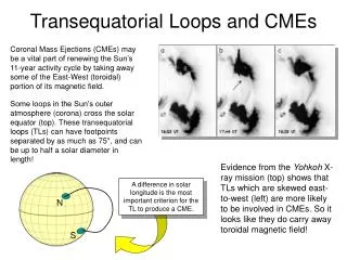
Transequatorial loops • Important component of the Babcock model – clues to the dynamo • CME association (e.g. Khan & Hudson, 2000, Glover et al. 2003) • Predicted to be formed by reconnection
Reconnection? • We saw an increase in intensity along with a cusp feature in SXR with (apparently) open field lines visible in EUV followed be a CME – consistent with the ‘standard’ LDE scenario. • First observation of a TEL at < 1 MK, velocities show mostly downflows (cooling).
Properties of coronal waves • From a study of 21 waves, 19 were associated with type II radio emission (Klassen et al., 2000). • Seen in the EUV and soft X-ray • Typical speed ~200-350 km/s (EUV), 600km/s (SXR). • Frequently associated with flares. • Often associated with CMEs (Biesecker et al., 2002). • Bright front followed by a large region of dimming.
13:28 14:00 14:12 14:53 14:21 14:35 • Fast mode shock wave related to a flare (e.g Uchida’s work)? • Shock wave caused by a fast CME? • Opening of field lines related to a CME (e.g. Delannee and Aulanier)?
First Spectroscopic Observation of Dimming • Synoptic CDS observation observed the dark region behind a wave front. Blue shifted velocities were observed (Harra & Sterling, 2001)
Two wave fronts are seen • No motion from either wave front is seen in CDS • The dimming region does not enter the CDS FOV! • Filament eruption seen
Filament eruption associated with wave This figure shows images at a 300 km/s blue shift. This feature is not obvious in the images alone. O v difference High v component Low v component
Explanation? • Chen et al. (2002) carried out 2D simulation of a piston-driven shock. • Our bright wave front could be their ‘EIT wave front’. • Our dimming region the density rareified region with strong expansion velocities. • They suggest that the ‘EIT’ wave result from opening of field lines associated with a filament eruption.