Turing Machines
Turing Machines. Chapter 17. Languages and Machines. SD D Context-Free Languages Regular Languages reg exps FSMs cfgs PDAs unrestricted grammars Turing Machines. Grammars, SD Languages, and Turing Machines. SD Language. L. Unrestricted Grammar. Accepts. Turing Machine.

Turing Machines
E N D
Presentation Transcript
Turing Machines Chapter 17
Languages and Machines SD D Context-Free Languages Regular Languages reg exps FSMs cfgs PDAs unrestricted grammars Turing Machines
Grammars, SD Languages, and Turing Machines SD Language L Unrestricted Grammar Accepts Turing Machine
Turing Machines • Can we come up with a new kind of automaton that has two properties: • ● powerful enough to describe all computable things • unlike FSMs and PDAs. • ● simple enough that we can reason formally about it • like FSMs and PDAs, • unlike real computers.
Turing Machines • At each step, the machine must: • ● choose its next state, • ● write on the current square, and • ● move left or right.
A Formal Definition A Turing machine M is a sextuple (K, , , , s, H): ● K is a finite set of states; ● is the input alphabet, which does not contain q; ● is the tape alphabet, which must contain q and have as a subset. ● sK is the initial state; ● HK is the set of halting states; ● is the transition function: (K - H) to K {, } non-halting tape state tape action state char char (R or L)
Notes on the Definition 1. The input tape is infinite in both directions. 2. is a function, not a relation. So this is a definition for deterministic Turing machines. 3. must be defined for all state, input pairs unless the state is a halting state. 4. Turing machines do not necessarily halt (unlike FSM's and PDAs). Why? To halt, they must enter a halting state. Otherwise they loop. 5. Turing machines generate output so they can compute functions.
An Example M takes as input a string in the language: {aibj, 0 ji}, and adds b’s as required to make the number of b’s equal the number of a’s. The input to M will look like this: The output should be:
The Details K = {1, 2, 3, 4, 5, 6}, = {a, b}, = {a, b, q, $, #}, s = 1, H = {6}, = If q is under r/w head, write q and move to right Hunt for unprocessed a Hunt for unprocessed b b found, go back Input is empty no more b, go back no more a, ready for changing $ to a and # to b
Notes on Programming The machine has a strong procedural feel, with one phase coming after another. There are common idioms, like scan left until you find a blank There are two common ways to scan back and forth marking things off. Often there is a final phase to fix up the output. Even a very simple machine is a nuisance to write.
Halting ● A DFSM M, on input w, is guaranteed to halt in |w| steps. ● A PDA M, on input w, is not guaranteed to halt. To see why, consider again M = But there exists an algorithm to construct an equivalent PDA M that is guaranteed to halt. A TM M, on input w, is not guaranteed to halt. And there exists no algorithm to construct one that is guaranteed to do so.
Formalizing the Operation A configuration of a Turing machine M = (K, , , s, H) is an element of: K ((- {q}) *) {} (* (- {q})) {} state up scanned after to scanned square scanned square square (left to r/w head) (under r/w head) (right to r/w head)
Example Configurations (1) (q, ab, b, b) = (q, abbb) (2) (q, , q, aabb) = (q, qaabb) Initial configuration is (s, qw).
Yields (q1, w1) |-M (q2, w2) iff (q2, w2) is derivable, via , in one step. For any TM M, let |-M* be the reflexive, transitive closure of |-M. Configuration C1yields configuration C2 if: C1|-M*C2. A path through M is a sequence of configurations C0, C1, …, Cn for some n 0 such that C0 is the initial configuration and: C0 |-MC1 |-MC2 |-M … |-MCn. A computation by M is a path that halts. If a computation is of lengthn or has n steps, we write: C0 |-MnCn
A Notation for Turing Machines (1) Define some basic machines ● Symbol writing machines For each x, define Mx, written just x, to be a machine that writes x “without moving” actually 2 steps ● Head moving machines R: rewrite whatever on the tape and move to right L: rewrite whatever on the tape and move to left ● Machines that simply halt: h, which simply halts (we don’t care about accept or reject) n, which halts and rejects y, which halts and accepts
Checking Inputs and Combining Machines Next we need to describe how to: ● Check the tape and branch based on what character we see, and ● Combine the basic machines to form larger ones. To do this, we need two forms: ● M1M2 ● M1 <condition> M2
A Notation for Turing Machines, Cont'd Example: >M1aM2 b M3 ● Start in the start state of M1. ● Compute until M1 reaches a halt state. ● Examine the tape and take the appropriate transition. ● Start in the start state of the next machine, etc. ● Halt if any component reaches a halt state and has no place to go. ● If any component fails to halt, then the entire machine may fail to halt.
Shorthands a M1M2 becomes M1a, bM2 b M1all elems of M2 becomes M1M2 or M1M2 Variables M1all elems of M2 becomes M1xaM2 except a and x takes on the value of the current square M1a, bM2 becomes M1xa, bM2 and x takes on the value of the current square M1x = yM2 if x = y then take the transition e.g., > xqRx if the current square is not blank, go right and copy it.
Some Useful Machines Find the first blank square to the right of the current square. Find the first blank square to the left of the current square. Find the first nonblank square to the right of the current square. Find the first nonblank square to the left of the current square Rq Lq Rq Lq
More Useful Machines La Find the first occurrence of a to the left of the current square. Ra,b Find the first occurrence of a or b to the right of the current square. La,baM1 Find the first occurrence of a or b to the left of the current square, b then go to M1 if the detected character is a; go to M2 if the M2 detected character is b. Lxa,b Find the first occurrence of a or b to the left of the current square and set x to the value found. Lxa,bRx Find the first occurrence of a or b to the left of the current square, set x to the value found, move one square to the right, and write x (a or b).
An Example Input: qww {1}* Output: qw3 Example: Input: q111qq Output: q111111111qq
A Shifting Machine S Input: quqwq Output: quwq Example: Input: qbaqabbaqq Output: qbaabbaqqq
Turing Machines as Language Recognizers Convention: We will write the input on the tape as: qwq, w contains no qs The initial configuration of M will then be: (s, qw) Let M = (K, , , , s, {y, n}). ● Maccepts a string w iff (s, qw) |-M* (y, w) for some string w. ● Mrejects a string w iff (s, qw) |-M* (n, w) for some string w.
Turing Machines as Language Recognizers Mdecides a language L* iff: For any string w * it is true that: if wL then M accepts w, and if wL then M rejects w. A language L is decidableiff there is a Turing machine M that decides it. In this case, we will say that L is in D.
A Deciding Example AnBnCn = {anbncn : n 0} Example: qaabbccqqqqqqqqq Example: qaaccbqqqqqqqqq
Another Deciding Example WcW = {wcw : w {a, b}*} Example: qabbcabbqqq Example: qacabbqqq
Semideciding a Language Let M be the input alphabet to a TM M. Let LM*. MsemidecidesL iff, for any string wM*: ● wLM accepts w ● wLM does not accept w. M may either: reject or fail to halt. A language L is semidecidable iff there is a Turing machine that semidecides it. We define the set SD to be the set of all semidecidable languages.
Example of Semideciding • Let L = b*a(ab)* • We can build M to semidecide L: • 1. Loop • 1.1 Move one square to the right. If the character under • the read head is an a, halt and accept. • In our macro language, M is:
Example of Semideciding • L = b*a(ab)*. We can also decide L: • Loop: • 1.1 Move one square to the right. • 1.2 If the character under the read/write head is • an a, halt and accept. • 1.3 If it is q, halt and reject. • In our macro language, M is:
Computing Functions Let M = (K, , , , s, {h}). Its initial configuration is (s, qw). Define M(w) = z iff (s, qw) |-M* (h, qz). Let be M’s output alphabet. Let f be any function from * to *. Mcomputesf iff, for all w*: ● If w is an input on which f is defined: M(w) = f(w). ● Otherwise M(w) does not halt. A function f is recursive or computable iff there is a Turing machine M that computes it and that always halts.
Example of Computing a Function Let = {a, b}. Let f(w) = ww. Input: qwqqqqqq Output: qwwq Define the copy machine C: qwqqqqqqqwqwq Remember the S machine: quqwqquwq Then the machine to compute f is just >CSLq
Example of Computing a Function Let = {a, b}. Let f(w) = ww. Input: qwqqqqqq Output: qwwq Define the copy machine C: qwqqqqqqqwqwq Remember the S machine: quqwqquwq Then the machine to compute f is just >CSLq
Computing Numeric Functions For any positive integer k, valuek(n) returns the nonnegative integer that is encoded, base k, by the string n. For example: ● value2(101) = 5. ● value8(101) = 65. TM M computes a function f from ℕm to ℕ iff, for some k: valuek(M(n1;n2;…nm)) = f(valuek(n1), … valuek(nm)).
Computing Numeric Functions Example: succ(n) = n + 1 We will represent n in binary. So n 01{0, 1}* Input: qnqqqqqq Output: qn+1q q1111qqqq Output: q10000q
Computing Numeric Functions Example: succ(n) = n + 1 We will represent n in binary. So n 01{0, 1}* Input: qnqqqqqq Output: qn+1q q1111qqqq Output: q10000q
Why Are We Working with Our Hands Tied Behind Our Backs? Turing machines Are more powerful than any of the other formalisms we have studied so far. Turing machines Are a lot harder to work with than all the real computers we have available. Why bother? The very simplicity that makes it hard to program Turing machines makes it possible to reason formally about what they can do. If we can, once, show that anything a real computer can do can be done (albeit clumsily) on a Turing machine, then we have a way to reason about what real computers can do.
Turing Machine Extensions There are many extensions we might like to make to our basic Turing machine model. But: We can show that every extended machine has an equivalent basic machine. Some possible extensions: ● Multiple tape TMs ● Nondeterministic TMs
Adding Tapes Adds No Power Theorem: Let M be a k-tape Turing machine for some k 1. Then there is a standard TM M' where ', and: ● On input x, M halts with output z on the first tape iff M' halts in the same state with z on its tape. ● On input x, if M halts in n steps, M' halts in O(n2) steps. Proof: By construction.
Impact of Nondeterminism • ● FSMs • ● Power NO • ● Complexity • Time NO • Space YES • ● PDAs • ● Power YES • ● Turing machines • ● Power NO • ● Complexity ?
Equivalence of Deterministic and Nondeterministic Turing Machines Theorem: If a nondeterministic TM M decides or semidecides a language, or computes a function, then there is a standard TM M' semideciding or deciding the same language or computing the same function. Proof: (by construction). We must do separate constructions for deciding/semideciding and for function computation.