1. System Analysis through Bond Graph Modeling Robert McBride May 3, 2005

2. Overview • Modeling • Bond Graph Basics • Bond Graph Construction • Simulation • System Analysis • Efficiency Definition and Analysis • Optimal Control • System Parameter Variation • Conclusions • References

3. Modeling: Bond Graph Basics • Bond graphs provide a systematic method for obtaining dynamic equations. • Based on the 1st law of thermodynamics. • Map the power flow through a system. • Especially suited for systems that cross multiple engineering domains by using a set of generic variables. • For an nth order system, bond-graphs naturally produce n, 1st-order, coupled equations. • This method easily identifies structural singularities in the model. Algebraic loops can also be identified.

4. e B A f Power moves from system A to system B Modeling: Bond Graph Basic Elements • The Power Bond • The most basic bond graph element is the power arrow or bond. • There are two generic variables associated with every power bond, e=effort, f=flow. • e*f = power.

5. Modeling: Bond Graph Basics • effort/flow definitions in different engineering domains

6. 5 4 0 1 1 11 3 13 2 12 Efforts are equal e1 = e2 = e3 = e4 = e5 Flows are equal f11 = f12 = f13 Flows sum to zero f1+ f2 = f3 + f4 + f5 Efforts sum to zero e11+ e12 = e13 Modeling: Bond Graph Basic Elements • Power Bonds Connect at Junctions. • There are two types of junctions, 0 and 1.

7. I C R e1 e2 e2 = 1/m*e1 TF f1 = 1/m*f2 f1 f2 m e1 e2 f2 = 1/d*e1 GY f1 = 1/d*e2 f1 f2 d SF SE Modeling: Bond Graph Basic Elements • I for elect. inductance, or mech. Mass • C for elect. capacitance, or mech. compliance • R for elect. resistance, or mech. viscous friction • TF represents a transformer • GY represents a gyrator • SE represents an effort source. • SF represents a flow source.

8. R:R1 R:R2 SE 0 1 1 SineVoltage1 C:C1 I:L1 Modeling: Bond Graph Construction This bond graph is a-causal

9. e f e f Modeling: Bond Graph ConstructionCausality • Causality determines the SIGNAL direction of both the effort and flow on a power bond. • The causal mark is independent of the power-flow direction.

10. e e I f f 1 1 e sI sC e C f f Modeling: Bond Graph ConstructionIntegral Causality Integral causality is preferred when given a choice.

11. Modeling: Bond Graph ConstructionNecessary Causality 5 4 0 1 1 11 3 13 2 12 f e Efforts are equal Flows are equal e1 = e3 = e4 = e5 ≡ e2 f11 = f13 ≡ f12

12. Modeling: Bond Graph Construction R:R1 R:R2 SE 0 1 1 SineVoltage1 C:C1 I:L1 This bond graph is Causal

13. Power flow through systems of complex geometry is often difficult to visualize. Force balancing methods may also be awkward due to the complexity of internal reaction forces. It is common to model these systems using an energy balance approach, e.g. a Lagrangian approach. Modeling: Bond Graph Construction From the System Lagrangian Question: Is there a method for mapping the Lagrangian of a system to a bond graph representation?

14. Assume that the system is conservative. Note the flow terms in the Lagrangian. The kinetic energy terms in the Lagrangian will have the form ½ I * f 2 where I is an inertia term and f is a flow term. Assign bond graph 1-junctions for each distinct flow term in the Lagrangian found in step 2. Note the generalized momentum terms. For each generalized momentum equation solve for the generalized velocity. Modeling: Lagrangian Bond Graph Construction

15. Note the equations derived from the Lagrangian show the balance of efforts around each 1-junction. If needed, develop the Hamiltonian for the conservative system. Add non-conservative elements where needed on the bond graph structure. Add external forces where needed as bond graph sources. Use bond graph methods to simplify if desired. Modeling: Lagrangian Bond Graph Construction (cont.)

16. Modeling: Lagrangian Bond Graph, Gyroscope Example

17. Modeling: Lagrangian Bond Graph, Gyroscope Example • The system is already conservative. • Rewrite the Lagrangian to note the flow terms. • Form 1-junctions for θ, ψ, and φ. • Generalized momentums are . . .

18. Modeling: Lagrangian Bond Graph, Gyroscope Example • Solve for the generalized velocities.

19. Modeling: Lagrangian Bond Graph, Gyroscope Example • Complete Lagrange Equations . . Note P*f Cross Terms

20. Modeling: Lagrangian Bond Graph, Gyroscope Example . .

21. Overview • Modeling • Bond Graph Basics • Bond Graph Construction • Simulation • System Analysis • Efficiency Definition and Analysis • Optimal Control • System Parameter Variation • Conclusions • References

22. Common Bond Graph Simulation Flow Chart Question: Does Such a Simulation Environment Exist? Bond Graph Construction Equation Formulation Simulation Environment Simulation Code Development Model Analysis through Simulation

23. The Dymola Simulation Environment • Dymola/Modelica provides an object-oriented simulation environment. • Dymola is very capable of handling algebraic loops and structural singularities. • Dymola does not have any knowledge of bond graph modeling. A bond graph library is needed within the framework of Dymola.

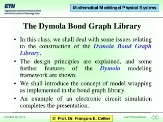
24. The Dymola Bond Graph Library • The bond graph library consists of a Dymola model for each of the basic bond graph elements. • These elements are used in an object-oriented manner to create bond graphs.

25. The Dymola Bond Graph Library: Bonds

26. The Dymola Bond Graph Library: Junctions

27. The Dymola Bond Graph Library: Passive Elements

28. The Dymola Gyroscope Bond Graph Model

29. The Dymola Gyroscope Bond Graph Model

30. Gyroscopically Stabilized Platform

31. Gyroscopically Stabilized Platform with Mounted Camera

32. Overview • Modeling • Bond Graph Basics • Bond Graph Construction • Simulation • System Analysis • Efficiency Definition and Analysis • Optimal Control • System Parameter Variation • Conclusions • References

33. System Analysis: Servo-Positioning System

34. System Analysis: Motor Dynamics

35. System Analysis: Fin Dynamics

36. System Analysis: Backlash Model

37. @ 6000 Hz @ 1200 Hz System Analysis: Servo Controllers Control Scheme 1 Control Scheme 2

38. System Analysis: Servo Step Response

39. System Analysis:Controller Efficiency Definition • By monitoring the output power and normalizing by the input power an efficiency calculations is defined as • Bond graph modeling naturally provides the means for this analysis.

40. System Analysis: Servo Step Response Efficiency

41. System Analysis:Controller Efficiency • The power flow through a bond graph model of the plant can be used to compare the effectiveness of different control schemes regardless of the architecture of the controller design, and without limiting the analysis to linear systems. Question: Can the controller efficiency be used to measure optimality of controller gain selection?

42. System Analysis: Missile System

43. System Analysis: Missile System Bond Graph

44. 1 1 1 System Analysis: Missile System 3-Loop Autopilot

45. System Analysis: Missile System Dymola Model

46. 0 0 Missile System Analysis: Performance Index Minimization Linear Constraints

47. Missile System Analysis: Performance Index Minimization δ α . θ = q

48. Sample Optimal Control Gains and Response

49. Sample Optimal Gain Efficiency

50. System Analysis:Controller Efficiency • The efficiency signal can be used as a benchmark when comparing efficiencies of different gain selections. • Constraint violation is assumed when the efficiency signal is more proficient than the benchmark. Question: How do the efficiency signals compare against an optimal control autopilot such as an SDRE design?