The Case For Prediction-based Best-effort Real-time
270 likes | 410 Vues
The Case For Prediction-based Best-effort Real-time. Peter A. Dinda Bruce Lowekamp Loukas F. Kallivokas David R. O’Hallaron Carnegie Mellon University. Overview. Distributed interactive applications Could benefit from best-effort real-time

The Case For Prediction-based Best-effort Real-time
E N D
Presentation Transcript
The Case For Prediction-based Best-effort Real-time Peter A. Dinda Bruce Lowekamp Loukas F. Kallivokas David R. O’Hallaron Carnegie Mellon University
Overview • Distributed interactive applications • Could benefit from best-effort real-time • Example: QuakeViz (Earthquake Visualization) and the DV (Distributed Visualization) framework • Evidence for feasibility of prediction-based best-effort RT service for these applications • Mapping algorithms • Execution time model • Host load prediction
Application Characteristics • Interactivity • Users initiate tasks with deadlines • Timely, consistent, and predictable feedback • Resilience • Missed deadlines are acceptable • Distributability • Tasks can be initiated on any host • Adaptability • Task computation and communication can be adjusted Shared, unreserved computing environments
Motivation for QuakeViz Teora, Italy 1980
Northridge Earthquake Simulation Real Event High Perf. Simulation 40 seconds of an aftershock of Jan 17, 1994 Northridge quake in San Fernando Valley of Southern California 16,666 40M x 40M SMVPs 15 GBytes of RAM 6.5 hours on 256 T3D PEs 80 trillion (1012) FLOPs 3.5 sustained GFLOP/s 1.4 peak GB/s Huge Model 50 x 50 x 10 km region 13,422,563 nodes 76,778,630 tetrahedrons 1 Hz frequency resolution 20 meter spatial resolution HUGE OUTPUT 16,666 time steps 13,422,563 3-tuples per step 6 Terabytes
Must Visualize Massive Remote Datasets Datasets must be kept at remote supercomputing site due to their sheer size Visualization is inherently distributed Problem One Month Turnaround Time
QuakeViz: Distributed Interactive Visualizationof Massive Remote Earthquake Datasets Sample 2 host visualization of Northridge Earthquake Goal Interactive manipulation of massive remote datasets from arbitrary clients
DV: A Framework For Building Distributed Interactive Visualizations of Massive Remote Datasets • Logical View: Distributed pipelines of vtk* modules • Example: local display and user User feedback and quality settings resolution contours ROI interpolation isosurface extraction Dataset reading rendering scene synthesis interpolation morphology reconstruction Display update latency deadline *Visualization Toolkit, open source C++ library
DV: A Framework For Building Distributed Interactive Visualizations of Massive Remote Datasets • Logical View: Distributed pipelines of vtk* modules • Example: local display and user User feedback and quality settings resolution contours ROI interpolation isosurface extraction Dataset reading rendering scene synthesis interpolation morphology reconstruction Display update latency deadline *Visualization Toolkit, open source C++ library
Active Frames Physical View of Example Pipeline: interpolation isosurface extraction scene synthesis deadline deadline deadline Active Frame n+2 ? Active Frame n+1 ? Active Frame n ? • Encapsulates data, computation, and path through pipeline • Launched from server by user interaction • Dynamically chose on which host each pipeline stage will execute and what quality settings to use
Active Frames Physical View of Example Pipeline: interpolation isosurface extraction scene synthesis deadline deadline deadline Active Frame n+2 ? Active Frame n+1 ? Active Frame n ? • Encapsulates data, computation, and path through pipeline • Launched from server by user interaction • Dynamically chose on which host each pipeline stage will execute and what quality settings to use
Active Frame Execution Model deadline Active Frame • pipeline stage • quality params Resource Predictions Mapping Algorithm Exec Time Model CMU Remos API Prediction Prediction Network Measurement Host Load Measurement Remos Measurement Infrastructure
Active Frame Execution Model deadline Active Frame • pipeline stage • quality params Resource Predictions Mapping Algorithm Exec Time Model CMU Remos API Prediction Prediction Network Measurement Host Load Measurement Remos Measurement Infrastructure
Active Frame Execution Model deadline Active Frame • pipeline stage • quality params Resource Predictions Mapping Algorithm Exec Time Model CMU Remos API Prediction Prediction Network Measurement Host Load Measurement Remos Measurement Infrastructure
Active Frame Execution Model deadline Active Frame • pipeline stage • quality params Resource Predictions Mapping Algorithm Exec Time Model CMU Remos API Prediction Prediction Network Measurement Host Load Measurement Remos Measurement Infrastructure
Active Frame Execution Model deadline Active Frame • pipeline stage • quality params Resource Predictions Mapping Algorithm Exec Time Model CMU Remos API Prediction Prediction Network Measurement Host Load Measurement Remos Measurement Infrastructure
Why Is Prediction Important? Bad Prediction No obvious choice Good Prediction Two good choices Predicted Exec Time Predicted Exec Time deadline Good predictions result in smaller confidence intervals Smaller confidence intervals simplify mapping decision
Comparing Prediction Models Run 1000s of randomized testcases, measure prediction error for each, datamine results: Inconsistent low error Consistent high error 97.5% Mean Squared Error 75% Consistent low error Mean 50% 25% Model A Model B Model C 2.5% Good models achieve consistently low error
Comparing Linear Models for Host Load Prediction 15 second predictions for one host 97.5% 75% Mean 50% 25% 2.5% Raw Very $ Cheap Expensive
Conclusions • Identified and described class of applicationsthat benefit from best-effort real-time • Distributed interactive applications • Example: QuakeViz / DV • Showed feasibility of prediction-based best-effort real-time systems • Mapping algorithms, execution time model, host load prediction
Status - http://www.cs.cmu.edu/~cmcl • QuakeViz / DV • Overview: PDPTA'99, Aeschlimann, et al • http://www.cs.cmu.edu/~quake • Currently under construction • Remos • Overview: HPDC’98, DeWitt, et al • Available from http://www.cs.cmu.edu/~cmcl/remulac/remos.html • Integrating prediction services • Network measurement and analysis • HPDC’98, DeWitt, et al; HPDC’99, Lowekamp, et al • Currently studying network prediction • Host load measurement and analysis • LCR’98, Dinda; SciProg’99, Dinda • Host load prediction • HPDC’99, Dinda, et al
Comparing Linear Models for Host Load Prediction 15 second predictions aggregated over 38 hosts 97.5% 75% Mean 50% 25% 2.5% Raw Very $ Cheap Expensive