Synchronization in Distributed Systems

SynchronizationinDistributed Systems Chapter 6

Guide to Synchronization Lectures • Synchronization in shared memory systems (2/19/09) • Event ordering in distributed systems (2/24) • Logical time, logical clocks, time stamps, • Mutual exclusion in distributed systems (2/26) • Election algorithms (3/3) • Data race detection in multithreaded programs (3/5)

Background • Synchronization: coordination of actions between processes. • Processes are usually asynchronous, (operate without regard to events in other processes) • Sometimes need to cooperate/synchronize • For mutual exclusion • For event ordering (was message x from process P sent before or after message y from process Q?)

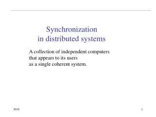
Introduction • Synchronization in centralized systems is primarily accomplished through shared memory • Event ordering is clear because all events are timed by the same clock • Synchronization in distributed systems is harder • No shared memory • No common clock

Clock Synchronization • Some applications rely on event ordering to be successful • See page 232 for some examples • Event ordering is easy if you can accurately time stamp events, but in a distributed system the clocks may not always be synchronized

Physical Clocks - pages 233-238 • Physical clock example: counter + holding register + oscillating quartz crystal • The counter is decremented at each oscillation • Counter interrupts when it reaches zero • Reloads from the holding register • Interrupt = clock tick (often 60 times/second) • Software clock: counts interrupts • This value represents number of seconds since some predetermined time (Jan 1, 1970 for UNIX systems; beginning of the Gregorian calendar for Microsoft) • Can be converted to normal clock times

Clock Skew • In a distributed system each computer has its own clock • Each crystal will oscillate at slightly different rate. • Over time, the software clock values on the different computers are no longer the same. • Clock skew: the difference in time values between different physical clocks • If an application expects the time associated with a file, message, or other object to be correct (independently of its local clock), clock skew can lead to failure.

Various Ways of Measuring Time • The sun • Mean solar second – gradually getting longer • International Atomic Time (TAI) • Atomic clocks are based on transitions of the cesium atom • Atomic second = value of solar second at some fixed time (no longer accurate) • Universal Coordinated Time (UTC) • Based on TAI seconds, but more accurately reflects sun time (inserts leap seconds)

Getting the Correct (UTC) Time • WWV radio station or similar stations in other countries (accurate to +/- 10 msec) • UTC services provided by earth satellites (accurate to .5 msec) • GPS (Global Positioning System) (accurate to 20-35 nanoseconds)

Clock Synchronization Algorithms • In a distributed system one machine may have a WWV receiver and some technique is used to keep all the other machines in synch with this value. • Or, no machine has access to an external time source and some technique is used to keep all machines synchronized with each other, if not with “real” time.

Clock Synchronization Algorithms • Network Time Protocol (NTP): • Objective: to keep all clocks in a system synchronized to UTC time (1-50 msec accuracy) • Uses a hierarchy of passive time servers • The Berkeley Algorithm: • Objective: to keep all clocks in a system synchronized to each other (internal synchronization) • Uses active time servers that poll machines periodically • Reference broadcast synchronization (RBS) • Objective: to keep all clocks in a wireless system synchronized to each other

Three Philosophies of Clock Synchronization • Try to keep all clocks synchronized to “real” time as closely as possible • Try to keep all clocks synchronized to each other, even if they vary somewhat from UTC time • Try to synchronize enough so that interacting processes can determine an event order. • Refer to these “clocks” as logical clocks

6.2 Logical Clocks • Observation: if two processes (running on separate processors) do not interact, it doesn’t matter if their clocks are not synchronized. • Observation: When processes do interact, they are usually interested in event order, instead of exact event time. • Conclusion: Logical clocks are sufficient for many applications

Lamport’s Logical Time • Leslie Lamport suggested the following method to order events in a distributed system. • "Events" are defined by the application. The granularity may be as coarse as a procedure or as fine-grained as a single instruction.

Formalization • The distributed system consists of n processes, p1, p2, …pn (e.g, a MPI group) • Each pi executes on a separate processor • No shared memory • Each pi has a state si • Process execution: a sequence of events • Changes to the local state • Message Send or Receive

Happened Before Relation (a b) • a  b: (page 244-245) • in the same [sequential] process/thread, • in different processes, (messages) • transitivity: if a  b and b  c, then a  c • Causally related events: • Event a may causally affect event b if a  b • Events a and b are causally related if either a  b or b  a.

Concurrent Events • Happened-before defines a partial order of events in a distributed system. • Some events can’t be placed in the order • a and b are concurrent (a || b) if !(a  b) and !(b  a). • If a and b aren’t connected by the happened-before relation, there’s no way one could affect the other.

Logical Clocks • Needed: method to assign a timestamp to event a (call it C(a)), even in the absence of a global clock • The method must guarantee that the clocks have certain properties, in order to reflect the definition of happens-before. • Define a clock (event counter), Ci, at each process (processor) Pi. • When an event a occurs, its timestamp ts(a) = C(a), the local clock value at the time the event takes place.

Correctness Conditions • If a and b are in the same process, anda  b then C(a) < C(b) • If a is the event of sending a message from Pi, and b is the event of receiving the message by Pj, then Ci (a) < Cj (b). • The value of C must be increasing (time doesn’t go backward). • Corollary: any clock corrections must be made by adding a positive number to a time.

Implementation Rules • For any two successive events a & b in Pi, increment the local clock (Ci = Ci + 1) • thus Ci(b) = Ci(a) + 1 • When a message m is sent, set its time-stamp tsm to Ci, the time of the send event after following previous step. • When the message is received the local time must be greater than tsm . The rule is (Cj = max{Cj, tsm} + 1). • Clock management can be handled as a middleware protocol

Lamport’s Logical Clocks (2) Figure 6-9. (a) Three processes, each with its own clock. The clocks “run” at different rates. Event c: P3 sends m3 to P2 at t = 60Event d: P2 receives m3 at t = 56Do C(c) and C(d) satisfy the conditions? Event a: P1 sends m1 to P2 at t = 6, Event b: P2 receives m1 at t = 16.If C(a) is the time m1 was sent, and C(b) is the time m1 is received, do C(a) and C(b) satisfy the correctness conditions ?

Lamport’s Logical Clocks (3) Figure 6-9. (b) Lamport’s algorithm corrects the clocks.

Application Layer Deliver mi to application Application sends message mi Adjust local clock, Timestamp mi Adjust local clock Middleware layer Middleware sends message Message mi is received Network Layer Figure 6-10. The positioning of Lamport’s logical clocks in distributed systems

Figure 5.3 (Advanced Operating Systems,Singhal and Shivaratri) How Lamport’s logical clocks advance e12 e13 e14 e16 e11 e15 e17 P1 e24 e21 e22 e23 e25 P2 Which events are causally related? Which events are concurrent? eij represents event j on processor i

A Total Ordering Rule • A total ordering of events can be obtained if we ensure that no two events have the same timestamp. • Why? So all processors can agree on an unambiguous order • How? Attach process number to low-order end of time, separated by decimal point; e.g., event at time 40 at process P1 is 40.1

Figure 5.3 - Singhal and Shivaratri e12 e13 e14 e16 e11 e15 e17 P1 e24 e21 e22 e23 e25 P2 What is the total ordering of the events in these two processes?

Example: Total Order Multicast • Consider a banking database, replicated across several sites. • Queries are processed at the geographically closest replica • We need to be able to guarantee that DB updates are seen in the same order everywhere

Totally Ordered Multicast Update 1: Process 1 at Site A adds $100 to an account, (initial value = $1000) Update 2: Process 2 at Site B increments the account by 1% Without synchronization,it’s possible thatreplica 1 = $1111,replica 2 = $1110

The Problem • Site 1 has final account balance of $1,111 after both transactions complete and Site 2 has final balance of $1,100. • Which is “right”? • Problem: lack of consistency. • Both values should be the same • Solution: make sure both sites see/process the messages in the same order.

Implementing Total Order • Assumptions: • Updates are multicast to all sites, including the sender • All messages from a single sender arrive in the order in which they were sent • No messages are lost • Messages are time-stamped with Lamport clock numbers

Implementation • When a process receives a message, put it in a local message queue, ordered by timestamp. • Multicast an acknowledgement to all sites • Each ack has a timestamp larger than the timestamponthemessage it acknowledges • The queue at each site will eventually be in the same order

Implementation • Deliver a message to the application only when the following conditions are true: • The message is at the head of the queue • The message has been acknowledged by all other receivers. • Acknowledgements are deleted when the message they acknowledge is processed. • Since all queues have the same order, all sites process the messages in the same order.

Vector Clock Rationale • Lamport clocks limitation: • If (ab) then C(a) < C(b) but • If C(a) < C(b) then we only know that either (ab) or (a || b), i.e., b a • In other words, you cannot look at the clock values of events on two different processors and decide which one comes first. • Lamport clocks do not capture causality

Figure 5.4 Time Space e11 . e12 P1 (2) (1) e21 e22 P2 (1) (3) e32 e31 e33 P3 (1) (2) (3) C(e11) < C(e22) and C(e11) < C(e32) but while e11 e22, we cannot say e11  e32 since there is no causal path connecting them. So, with Lamport clocks we can guarantee that if C(a) < C(b) then b a , but by looking at the clock values alone we cannot say whether or not the events are causally related.

Vector Clocks – How They Work • Each processor keeps a vector of values, instead of a single value. • VCi is the clock at process i; it has a component for each process in the system. • VCi[i] corresponds to Pi‘s local “time”. • VCi[j] represents Pi‘s knowledge of the “time” at Pj (the # of events that Pi knows have occurred at Pj • Each processor knows its own “time” exactly, and updates the values of other processors’ clocks based on timestamps received in messages.

Implementation Rules • IR1: Increment VCi[i] before each new event. • IR2: When process i sends a message m it sets m’s (vector) timestamp to VCi. • IR3: When a process receives a message it does a component-by-component comparison of the message timestamp to its local time and picks the maximum of the two corresponding components. • Then deliver the message to the application.

Figure 5.5. Singhal and Shivaratri (2, 0, 0) (3, 5, 2) (1, 0 , 0) P1 e11 e12 e13 (0, 1, 0) (2, 5, 2) (2,4,2) (2, 2, 0) (2, 3, 1) P2 e21 e22 e24 e25 e23 (0, 0, 1) (0, 0, 2) P3 e32 e31

Establishing Causal Order • If event a has timestamp ts(a), then ts(a)[i]-1 is the number of events at Pi that causally preceded a. • When Pi sends a message m to Pj, Pj knows • How many events occurred at Pi before m was sent • How many relevant events occurred at other sites before m was sent (relevant = “happened-before”) • In Figure 5.5, VC(e23) = (2, 3, 1). Two events in P1 and one event in P3 “happened before” e23. • Even though P1 and P3 may have executed other events, they don’t have a causal effect on e23.

Happened Before/Causally Related Events - Vector Clock Definition • Events a and b are causally related if • ts(a) < ts(b)or • ts(b) < ts(a) • Otherwise, we say the events are concurrent. • a → b iff ts(a) < ts(b)(a happens before b iff the timestamp of a is less than the timestamp of b) • Any pair of events that satisfy the vector clock definition of happens-before will also satisfy the Lamport definition, and vice-versa.

Comparing Vector Timestamps • Less than or equal: ts(a)≤ts(b) if each component of ts(a)[i] is ≤ ts(b)[i] • Equal: ts(a) = ts(b) iff every component in ts(a)[i] is equal to ts(b)[i]. (In this case a and b are the same events) • Less than: ts(a) < ts(b)iff ts(a) is less than or equal to ts(b), but ts(a) is not equal ts(b). In other words, at least one component of ts(a) is strictly less than the corresponding component of ts(b) . • Concurrent: ts(a) || ts(b) if ts(a) isn’t less than ts(b)and ts(b) isn’t less than ts(a).

Figure 5.4 Time e11 e12 P1 (2) (1) e21 e22 P2 (1) (3) e32 e31 e33 P3 (1) (2) (3) ts(e11) = (1, 0, 0) and ts(e32) = (0, 0, 2), which shows that the two events are concurrent. ts(e11) = (1, 0, 0) and ts(e22) = (2, 3, 0), which shows that e11 e22

Causal Ordering of Messages An Application of Vector Clocks • Premise: Deliver a message only if messages that causally precede it have already been received • i.e., if send(m1)  send(m2), then it should be true that receive(m1)  receive(m2) at each site. • If messages are not related (send(m1) || send(m2), delivery order is not of interest.

Compare to Total Order • Totally ordered multicast (TOM) is stronger (more inclusive) than causal ordering (COM). • TOM orders all messages, not just those that are causally related. • “Weaker” COM is often all that is needed.

Enforcing Causal Communication • Clocks are adjusted only when sending or receiving messages; i.e, these are the only events of interest. • Send m: Pi increments VCi[i] by 1 and applies timestamp, ts(m). • Receive m: Pi compares VCi to ts(m); set VCi[i] to max{VCi[i] , ts(m)[k]} for each k.

Message Delivery Conditions • Suppose: PJ receives message m from Pi • Middleware delivers m to the application iff • ts(m)[i] = VCj[i] + 1 • all previous messages from Pi have been delivered • ts(m)[k] ≤ VCi[k] for all k ≠ i • PJ has received all messages that Pi had seen before it sent message m.

In other words, if a message m is received from Pi, you should also have received every message that Pi received before it sent m; e.g., • if m is sent by P1 and ts(m) is (3, 4, 0) and you are P3, you should have received exactly 2 messages from P1 and at least 4 from P2 • if m is sent by P2 and ts(m) is (4, 5, 1, 3) and if you are P3 and VC3 is (3, 3, 4, 3) then you need to wait for a fourth message from P2 and at least one more message from P1.

Figure 6-13. Enforcing Causal Communication VC0 VC0 P0 (1, 0, 0) (1, 1, 0) m P1 (1, 1, 0) VC1 m* P2 (0, 0, 0) (1, 0, 0) (1, 1, 0) VC2 VC2 VC2 P1 received message m from P0 before sending message m* to P2; P2 must wait for delivery of m before receiving m* (Increment own clock only on message send) Before sending or receiving any messages, one’s own clock is (0, 0, …0)

History • ISIS and Horus were middleware systems that supported the building of distributed environments through virtually synchronous process groups • Provided both totally ordered and causally ordered message delivery. • “Lightweight Causal and Atomic Group Multicast” • Birman, K., Schiper, A., Stephenson, P, ACM Transactions on Computer Systems, Vol 9, No. 3, August 1991, pp 272-314.

Location of Message Delivery • Problems if located in middleware: • Message ordering captures only potential causality; no way to know if two messages from the same source are actually dependent. • Causality from other sources is not captured. • End-to-end argument: the application is better equipped to know which messages are causally related. • But … developers are now forced to do more work; re-inventing the wheel.

Revised Lecture Schedule • 10/14: Finished L12, started L13 • 10/16: L13 + start L14 • 10/21: L14 + L15 • 10/23: L16: Detecting Race Conditions in Multithreaded Programs. • This lecture is based on papers 10 and 11 from the reading list.

Synchronization in Distributed Systems