Analytic Geometry

Analytic Geometry Rene Descartes: Founder of Analytic Geometry Cartesian Coordinate System Graphing an equation Graphically finding solutions to equations

Cartesian coordinate plane is formed by two equal perpendicular lines. These lines are called axes. The y-axis is the vertical axis while the x-axis is the horizontal axis. y-axis x-axis origin The point where the axes intersect is known as the origin.

The Cartesian plane is divided into four quadrants.

Distances are measured from the origin along each axis. The distances are positive moving right along the x-axis and up along the y-axis. The distances are negative moving left along the x-axis and down along the y-axis. The distances continue to infinity along each axis in both directions.

The position of different points on the Cartesian plane is expressed in relation to first the horizontal distance and then the vertical distance from the origin. The horizontal distance is known as the x-coordinate. The vertical distance is known as the y-coordinate. The position is expressed as ordered pairs (x,y). The x-coordinate is always written first. The purple point is the origin. The green point is located 2 units right and 3 units up from the origin. The red point is located 3 units left and 1 unit up from the origin. The blue point is located 1.5 units left and 2.5 units down from the origin

City Map The Cartesian Plane can be viewed as a city map. A location within the city is indicated by street and avenue. The avenues would be the x-values. The streets would be the y-values. Street Avenue

The Cartesian plane is also used to show the relationship between two variables x and y by plotting multiple points on the plane. The relationship between the points on the graph below is that each time x moves one to the left, y moves three up.

A point on a graph is located in terms of where the y-coordinate is in relation to the x-coordinate. Thus, the y-coordinate is considered to be dependant on the x-coordinate. y-axis The x-axis is the independent variable. The y-axis is the dependent variable. x-axis

A curve can be drawn through all the points on a graph. It is called a curve even if the graph is in a straight line. The curve not only shows what y-coordinates are for each integer values of x (shown on the graph below) but also for the decimal values of x. The relationship between every value of x and y on the curve is the same.

The relationship represented by the curve of graph satisfies a mathematical equation. Any mathematical equation with two variables can be represented on the Cartesian plane. The curve on the graph below satisfies the equation y=x3. Putting any x-coordinate in the equation for x, the corresponding answer for y will be the same as the y-coordinate on the curve.

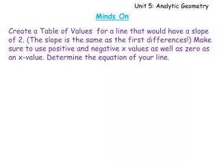
How to graph a mathematical equation on a Cartesian Plane? 1. Get a mathematical equation. 2. Create a Table of Values. To create a table of values, take a number of create a table with two columns with heading x and y. Put a number of integer values into the x-column. This should include zero and number of positive and negative numbers. Find y by putting the corresponding x values into the given equation. Example

Example • The equation is 3x-2=y • Create a Table of Values. 3. Select a number of positive and negative values for x, including zero. 4. Substitute these x values into the equation to get the corresponding y values. Click on this box to practice making Table of Values. Back

Graphing a mathematical equation continued 3. The different pairs of numbers in the Table of Values can now be plotted on the Cartesian Plane.

4. Before we can connect the points with a curve, we have to know what kind of curve it is going to be. Does it dip or curve between the points? Is it a straight line? Is there any places where the curve is undefined? The Highest Degree of the Equation will give the shape of the curve. Click on the buttons to view the different graphs. Linear Quadratic Cubic Quartic

Linear Equations • Degree: one • Shape of Curve: straight line • Simplest equation: y=x • Number x-intercepts: one Back

Quadratic Equations • Degree: two • Shape of Curve: parabola • Simplest Equation : y=x2 • Number of x-intercepts: two Back

Cubic Equations • Degree: three • Shape of Curve: shown below • Simplest Equation: y=x3 • Number of x-intercepts: three Back

Quartic Equations • Degree: four • Shape of Curve: shown below • Simplest Equation: y=x4 • Number of x-intercepts: four Back

The equation y=3x-2 is a linear equation so the curve is a straight line.

Explore what the curves of following forms of equations will look like. Click on the different equations. y= ax + b y= ax2 + bx +c y= ax3 + bx2 + cx + d y= ax4 + bx3 + cx2 +dx + e

X-Intercepts The place where the curve crosses the x-axis is called the x-intercept. This graph has two x-intercepts x-intercept x-intercept

X-Intercepts The x-axis is the line where all the y-coordinates are zero. This means that a x-intercept has a y-coordinate that is equal to zero. (2,0) (-4,0) (-1,0)

X-Intercepts The solutions of an equation are the values of x for when y=0. The x-intercepts are then the solutions of an equation. This is the graph of y=x2+3x-10 The x-intercepts are -5 and 2. Solving the Equation The solutions for y=x2+3x-10 are: =(-5)2+3(-5)-10 =25+(-15)-10 =0 =(2)2+3(2)-10 =4+6-10 =0 (2,0) (-5,0)

X-Intercepts The solutions of an equation can be solved graphically by finding the x-intercepts. Sometimes x-intercepts are whole numbers and can be observed from the graph but most times the x-intercepts falls between the whole number making it difficult to identify. Example below shows this. Graphing calculators have different functions that can be used to find the x-intercept

Analytic Geometry