Biological Risk Estimation for Leukemia Using Bayesian Inference and Gibbs Sampling

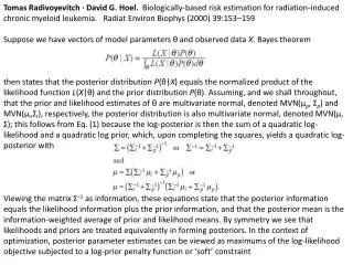
1. Tomas Radivoyevitch · David G. Hoel. Biologically-based risk estimation for radiation-induced chronic myeloid leukemia. RadiatEnviron Biophys (2000) 39:153–159 Suppose we have vectors of model parameters θ and observed data X. Bayes theorem then states that the posterior distribution P(θ|X) equals the normalized product of the likelihood function L(X|θ) and the prior distribution P(θ). Assuming, and we shall throughout, that the prior and likelihood estimates of θ are multivariate normal, denoted MVN(μp, Σp) and MVN(μl,Σl), respectively, the posterior distribution is also multivariate normal, denoted MVN(μ, Σ); this follows from Eq. (1) because the log-posterior is then the sum of a quadratic log-likelihood and a quadratic log prior, which, upon completing the squares, yields a quadratic log-posterior with Viewing the matrix Σ–1 as information, these equations state that the posterior information equals the likelihood information plus the prior information, and that the posterior mean is the information-weighted average of prior and likelihood means. By symmetry we see that likelihoods and priors are treated equivalently in forming posteriors. In the context of optimization, posterior parameter estimates can be viewed as maximums of the log-likelihood objective subjected to a log-prior penalty function or ‘soft’ constraint

2. Bayesian Inference using Gibbs Sampling (BUGS) version 0.5 Manual

3. Bayesian Inference using Gibbs Sampling (BUGS) version 0.5 Manual > LINE # name of this model in rjags JAGS model: model { for( i in 1 : N ) { Y[i] ~ dnorm(mu[i],tau) mu[i] <- alpha + beta * (x[i] - xbar) } tau ~ dgamma(0.001,0.001) sigma <- 1 / sqrt(tau) alpha ~ dnorm(0.0,1.0E-6) beta ~ dnorm(0.0,1.0E-6) } Fully observed variables: N Y x xbar