Declarative Programming Techniques
Declarative Programming Techniques. Seif Haridi KTH Peter Van Roy UCL. Overview. What is declarativeness? Classification, advantages for large and small programs Iterative and recursive programs Programming with lists and trees

Declarative Programming Techniques
E N D
Presentation Transcript
Declarative Programming Techniques Seif Haridi KTH Peter Van Roy UCL S. Haridi and P. Van Roy
Overview • What is declarativeness? • Classification, advantages for large and small programs • Iterative and recursive programs • Programming with lists and trees • Lists, accumulators, difference lists, trees, parsing, drawing trees • Reasoning about efficiency • Time and space complexity, big-oh notation, recurrence equations • Higher-order programming • Basic operations, loops, data-driven techniques, laziness, currying • User-defined data types • Dictionary, word frequencies • Making types secure: abstract data types • The real world • File and window I/O, large-scale program structure, more on efficiency • Limitations and extensions of declarative programming S. Haridi and P. Van Roy
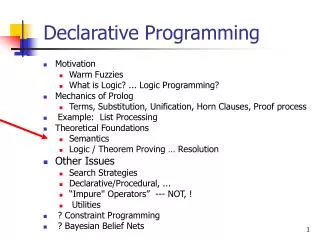
Declarative operations (1) • An operation is declarative if whenever it is called with the same arguments, it returns the same results independent of any other computation state • A declarative operation is: • Independent (depends only on its arguments, nothing else) • Stateless (no internal state is remembered between calls) • Deterministic (call with same operations always give same results) • Declarative operations can be composed together to yield other declarative components • All basic operations of the declarative model are declarative and combining them always gives declarative components S. Haridi and P. Van Roy
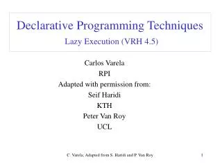
Arguments Declarativeoperation Results Declarative operations (2) rest of computation S. Haridi and P. Van Roy
Why declarative components (1) • There are two reasons why they are important: • (Programming in the large)A declarative component can be written, tested, and proved correct independent of other components and of its own past history. • The complexity (reasoning complexity) of a program composed of declarative components is the sum of the complexity of the components • In general the reasoning complexity of programs that are composed of nondeclarative components explodes because of the intimate interaction between components • (Programming in the small)Programs written in the declarative model are much easier to reason about than programs written in more expressive models (e.g., an object-oriented model). • Simple algebraic and logical reasoning techniques can be used S. Haridi and P. Van Roy
Why declarative components (2) • Since declarative components are mathematical functions, algebraic reasoning is possible i.e. substituting equals for equals • The declarative model of chapter 4 guarantees that all programs written are declarative • Declarative components can be written in models that allow stateful data types, but there is no guarantee S. Haridi and P. Van Roy
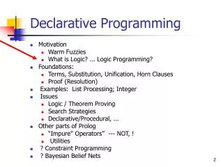
Classification ofdeclarative programming • The word declarative means many things to many people. Let’s try to eliminate the confusion. • The basic intuition is to program by defining the what without explaining the how Descriptive Declarativeprogramming Observational Functional programming Programmable Declarative model Deterministiclogic programming Definitional Nondeterministiclogic programming S. Haridi and P. Van Roy
Descriptive language s::= skip empty statement | x = y variable-variable binding | x = record variable-value binding | s1 s2 sequential composition | local x in s1 end declaration Other descriptive languages include HTML and XML S. Haridi and P. Van Roy
Descriptive language <person id = ”530101-xxx”> <name> Seif </name> <age> 48 </age> </person> Other descriptive languages include HTML and XML S. Haridi and P. Van Roy
Kernel language The following defines the syntax of a statement, sdenotes a statement s::= skip empty statement | x = y variable-variable binding | x = v variable-value binding | s1 s2 sequential composition | local x in s1 end declaration| proc {x y1 … yn } s1 end procedure introduction | if x then s1 else s2 end conditional | { x y1 … yn } procedure application | case x of pattern then s1 else s2 end pattern matching S. Haridi and P. Van Roy
Why the KL is declarative • All basic operations are declarative • Given the components (substatements) are declarative, • sequential composition • local statement • procedure definition • procedure call • if statement • try statement are all declarative S. Haridi and P. Van Roy
Structure of this chapter • Iterative computation • Recursive computation • Thinking inductively • Lists and trees data abstraction procedural abstraction • Control abstraction • Higher-order programming • User-defined data types • Secure abstract data types • Modularity • Functors and modules • Time and space complexity • Nondeclarative needs • Limits of declarative programming S. Haridi and P. Van Roy
Iterative computation • An iterative computation is a one whose execution stack is bounded by a constant, independent of the length of the computation • Iterative computation starts with an initial state S0, and transforms the state in a number of steps until a final state Sfinal is reached: S. Haridi and P. Van Roy
The general scheme fun {Iterate Si} if {IsDoneSi} thenSi elseSi+1in Si+1 = {TransformSi} {Iterate Si+1} end end • IsDoneand Transform are problem dependent S. Haridi and P. Van Roy
The computation model • STACK : [ R={Iterate S0}] • STACK : [ S1 = {Transform S0}, R={Iterate S1} ] • STACK : [ R={Iterate S1}] • STACK : [ Si+1 = {Transform Si}, R={Iterate Si+1} ] • STACK : [ R={Iterate Si+1}] S. Haridi and P. Van Roy
Newton’s method for thesquare root of a positive real number • Given a real number x, start with a guess g, and improve this guess iteratively until it is accurate enough • The improved guess g’ is the average of g and x/g: S. Haridi and P. Van Roy
Newton’s method for thesquare root of a positive real number • Given a real number x, start with a guess g, and improve this guess iteratively until it is accurate enough • The improved guess g’ is the average of g and x/g: • Accurate enough is defined as: | x – g2 | / x < 0.00001 S. Haridi and P. Van Roy
SqrtIter fun {SqrtIter Guess X} if {GoodEnough Guess X} then Guess else Guess1 = {Improve Guess X} in {SqrtIter Guess1 X} end end • Compare to the general scheme: • The state is the pair Guess and X • IsDone is implemented by the procedure GoodEnough • Transform is implemented by the procedure Improve S. Haridi and P. Van Roy
The program version 1 fun {Sqrt X} Guess = 1.0 in {SqrtIter Guess X} end fun {SqrtIter Guess X} if {GoodEnough Guess X} then Guess else {SqrtIter {Improve Guess X} X} end end fun {Improve Guess X} (Guess + X/Guess)/2.0 end fun {GoodEnough Guess X} {Abs X - Guess*Guess}/X < 0.00001 end S. Haridi and P. Van Roy
Using local procedures • The main procedure Sqrt uses the helper procedures SqrtIter, GoodEnough, Improve, and Abs • SqrtIter is only needed inside Sqrt • GoodEnough and Improve are only needed inside SqrtIter • Abs (absolute value) is a general utility • The general idea is that helper procedures should not be visible globally, but only locally S. Haridi and P. Van Roy
Sqrt version 2 local fun {SqrtIter Guess X} if {GoodEnough Guess X} then Guess else {SqrtIter {Improve Guess X} X} end end fun {Improve Guess X} (Guess + X/Guess)/2.0 end fun {GoodEnough Guess X} {Abs X - Guess*Guess}/X < 0.000001 end in fun {Sqrt X} Guess = 1.0 in {SqrtIter Guess X} end end S. Haridi and P. Van Roy
Sqrt version 3 • Define GoodEnough and Improve inside SqrtIter local fun {SqrtIter Guess X} fun {Improve} (Guess + X/Guess)/2.0 end fun {GoodEnough} {Abs X - Guess*Guess}/X < 0.000001 end in if {GoodEnough} then Guess else {SqrtIter {Improve} X} end end infun {Sqrt X} Guess = 1.0 in {SqrtIter Guess X} end end S. Haridi and P. Van Roy
Sqrt version 3 • Define GoodEnough and Improve inside SqrtIter local fun {SqrtIter Guess X} fun {Improve} (Guess + X/Guess)/2.0 end fun {GoodEnough} {Abs X - Guess*Guess}/X < 0.000001 end in if {GoodEnough} then Guess else {SqrtIter {Improve} X} end end infun {Sqrt X} Guess = 1.0 in {SqrtIter Guess X} end end The program has a single drawback: on each iteration two procedure values are created, one for Improve and one for GoodEnough S. Haridi and P. Van Roy
Sqrt final version fun {Sqrt X} fun {Improve Guess} (Guess + X/Guess)/2.0 end fun {GoodEnough Guess} {Abs X - Guess*Guess}/X < 0.000001 end fun {SqrtIter Guess} if {GoodEnough Guess} then Guess else {SqrtIter {Improve Guess} } end end Guess = 1.0 in {SqrtIter Guess} end The final version is a compromise between abstraction and efficiency S. Haridi and P. Van Roy
From a general schemeto a control abstraction (1) fun {Iterate Si} if {IsDoneSi} thenSi elseSi+1in Si+1 = {TransformSi} {Iterate Si+1} end end • IsDoneand Transform are problem dependent S. Haridi and P. Van Roy
From a general schemeto a control abstraction (2) fun {Iterate SIsDone Transform} if {IsDone S} then S else S1 in S1 = {Transform S} {Iterate S1} end end fun {Iterate Si} if {IsDoneSi} thenSi elseSi+1in Si+1 = {TransformSi} {Iterate Si+1} end end S. Haridi and P. Van Roy
Sqrt using the Iterate abstraction fun {Sqrt X} fun {Improve Guess} (Guess + X/Guess)/2.0 end fun {GoodEnough Guess} {Abs X - Guess*Guess}/X < 0.000001 end Guess = 1.0 in {Iterate Guess GoodEnough Improve} end S. Haridi and P. Van Roy
Sqrt using the Iterate abstraction fun {Sqrt X} {Iterate 1.0 fun {$ G} {Abs X - G*G}/X < 0.000001 end fun {$ G} (G + X/G)/2.0 end } end This could become a linguistic abstraction S. Haridi and P. Van Roy
Recursive computations • Recursive computation is one whose stack size grows linear to the size of some input data • Consider a secure version of the factorial function: fun {Fact N} if N==0 then 1 elseif N>0 then N*{Fact N-1} elseraise domainError end end end • This is similar to the definition we saw before, but guarded against domain errors (and looping) by raising an exception S. Haridi and P. Van Roy
Recursive computation proc {Fact N R} if N==0 then R=1 elseif N>0 then R1 in {Fact N-1 R} R = N*R1 elseraise domainError end end end S. Haridi and P. Van Roy
Execution stack • [{Fact 5 r0}] • [{Fact 4 r1} , r0=5* r1] • [{Fact 3 r2}, r1=4* r2 , r0=5* r1] • [{Fact 2 r3}, r2=3* r3 , r1=4* r2 , r0=5* r1] • [{Fact 1 r4}, r3=2* r4 , r2=3* r3 , r1=4* r2 , r0=5* r1] • [{Fact 0 r5}, r4=1* r5, r3=2* r4 , r2=3* r3 , r1=4* r2 , r0=5* r1] • [r5=1, r4=1* r5, r3=2* r4 , r2=3* r3 , r1=4* r2 , r0=5* r1] • [r4=1* 1, r3=2* r4 , r2=3* r3 , r1=4* r2 , r0=5* r1] • [r3=2* 1 , r2=3* r3 , r1=4* r2 , r0=5* r1] • [r2=3* 2 , r1=4* r2 , r0=5* r1] S. Haridi and P. Van Roy
Substitution-basedabstract machine • The abstract machine we saw in Chapter 4 is based on environments • It is nice for a computer, but awkward for hand calculation • We make a slight change to the abstract machine so that it is easier for a human to calculate with • Use substitutions instead of environments: substitute identifiers by their store entities • Identifiers go away when execution starts; we manipulate store variables directly S. Haridi and P. Van Roy
Iterative Factorial • State: {Fact N} • (0,{Fact 0}) (1,{Fact 1}) … (N,{Fact N}) • In general: (I,{Fact I}) • Termination condition: is I equal to Nfun {IsDone I FI } I == N end • Transformation : (I,{Fact I}) (I+1, (I+1)*{Fact I}) proc {Transform I FI I1 FI1} I1 = I+1 FI1 = I1*FIend S. Haridi and P. Van Roy
Iterative Factorial • State: {Fact N} • (0,{Fact 0}) (1,{Fact 1}) … (N,{Fact N}) • Transformation : (I,{Fact I}) (I+1, (I+1)*{Fact I}) • fun {FactN}fun {FactIter I FI}if I==N then FIelse {FactIter I+1 (I+1)*FI} endend {FactIter 0 1}end S. Haridi and P. Van Roy
Iterative Factorial • State: {Fact N} • (0,{Fact 0}) (1,{Fact 1}) … (N,{Fact N}) • Transformation : (I,{Fact I}) (I+1, (I+1)*{Fact I}) • fun {FactN} {Iterate t(0 1)fun {$ t(I IF)} I == N endfun {$ t(I IF)} J = I+1 in t(J J*IF) end }end S. Haridi and P. Van Roy
Iterative Factorial • State: {Fact N} • (1,5) (1*5,4) … ({Fact N},0) • In general: (I,J) • Invariant I*{Fact J} == (I*J)*{Fact J-1} == {Fact N} • Termination condition: is J equal to 0fun {IsDone I J} I == 0 end • Transformation : (I,J) (I*J, J-1) proc {Transform I J I1 J1} I1 = I*J J1 = J1-1end S. Haridi and P. Van Roy
Programmingwith lists and trees • Defining types • Simple list functions • Converting recursive to iterative functions • Deriving list functions from type specifications • State and accumulators • Difference lists • Trees • Drawing trees S. Haridi and P. Van Roy
User defined data types • A list is defined as a special subset of the record datatype • A list Xs is either • X|Xr where Xr is a list, or • nil • Other subsets of the record datatype are also useful, for example one may define a binary tree (btree) to be: • node(key:K value:V left:LT right:RT) where LT and BT are binary trees, or • leaf • This begs for a notation to define concisely subtypes of records S. Haridi and P. Van Roy
Defining types list ::= value | list [] nil • defines a list type where the elements can be of any type list T ::= T | list [] nil • defines a type function that given the type of the parameter T returns a type, e.g. list int btree T ::= node(key: literal value:T left: btree T right: btree T) [] leaf(key: literal value:T) • Procedure types are denoted by proc{T1 … Tn} • Function types are denoted by fun{T1 … Tn}:T and is equivalent to proc{T1 … Tn T} • Examples: fun{list list }: list S. Haridi and P. Van Roy
Lists • General Lists have the following definitionlist T ::= T | list [] nil • The most useful elementary procedures on lists can be found in the Base module List of the Mozart system • Induction method on lists, assume we want to prove a property P(Xs) for all lists Xs • The Basis: prove P(Xs) for Xs equals to nil, [X], and [X Y] • The Induction step: Assume P(Xs) hold, and prove P(X|Xs) for arbitrary X of type T S. Haridi and P. Van Roy
Constructive method forprograms on lists • General Lists have the following definitionlist T ::= T | list T [] nil • The task is to write a program {Task Xs1 … Xsn} • Select one or more of the arguments Xsi • Construct the task for Xsi equals to nil, [X], and [X Y] • The recursive step: assume {Task … Xsi …} is constructed, and design the program for {Task … X|Xsi …} for arbitrary X of type T S. Haridi and P. Van Roy
Simple functions on lists • Some of these functions exist in the library module List: • {Nth Xs N}, returns the Nth element of Xs • {Append Xs Ys}, returns a list which is the concatenation of Xs followed by Ys • {Reverse Xs} returns the elements of Xs in a reverse order, e.g. {Reverse [1 2 3]} is [3 2 1] • Sorting lists, MergeSort • Generic operations of lists, e.g. performing an operation on all the elements of a list, filtering a list with respect to a predicate P S. Haridi and P. Van Roy
The Nth function • Define a function that gets the Nth element of a list • Nth is of type fun{$ list T int}:T , • Reasoning: select N, two cases N=1, and N>1: • N=1: {Nth Xs 1} Xs.1 • N>1: assume we have the solution for {Nth Xr N-1} for a smaller list Xr, then {Nth X|Xr N} {Nth Xr N-1} fun {Nth Xs N}X|Xr = Xs in if N==1 then X elseif N>1 then {Nth Xr N-1} end end S. Haridi and P. Van Roy
The Nth function fun {Nth Xs N}X|Xr = Xs in if N==1 then X elseif N>1 then {Nth Xr N-1} end end • fun {Nth Xs N}if N==1 then Xs.1 • elseif N>1 then {Nth Xs.2 N-1} • end • end S. Haridi and P. Van Roy
The Nth function • Define a function that gets the Nth element of a list • Nth is of type fun{$ list T int}:T , fun {Nth Xs N} if N==1 then Xs.1 elseif N>1 then {Nth Xs.2 N-1} end end • There are two situations where the program fails: • N > length of Xs, (we get a situation where Xs is nil) or • N is not positive, (we get a missing else condition) • Getting the nth element takes time proportional to n S. Haridi and P. Van Roy
The Member function • Member is of type fun{$ valuelist value}:bool , fun {Member E Xs} case Xs of nil thenfalse [] X|Xr then if X==E thentrueelse {Member E Xr} end end end • X==E orelse {Member E Xr} is equivalent to • if X==E thentrueelse {Member E Xr} end • In the worst case, the whole list Xs is traversed, i.e., worst case behavior is the length of Xs, and on average half of the list S. Haridi and P. Van Roy
The Append function fun {Append Xs Ys} case Xs of nil then Ys [] X|Xr then X|{Append Xr Ys} end end • The inductive reasoning is on the first argument Xs • Appending Xs and Ys is proportional to the length of the first list • declare Xs0 = [1 2] Ys = [a b] Zs0 = {Append Xs0 Ys} • Observe that Xs0, Ys0 and Zs0 exist after Append • A new copy of Xs0, call it Xs0’, is constructed with an unbound variable attached to the end: 1|2|X’, thereafter X’ is bound to Ys S. Haridi and P. Van Roy
The Append function proc {Append Xs Ys Zs} case Xs of nil thenZs = Ys [] X|Xr thenZr in Zs = X|Zr {Append Xr Ys Zr} end end • declare Xs0 = [1 2] Ys = [a b] Zs0 = {Append Xs0 Ys} • Observe that Xs0, Ys and Zs0 exist after Append • A new copy of Xs0, call it Xs0’, is constructed with an unbound variable attached to the end: 1|2|X’, thereafter X’ is bound to Ys S. Haridi and P. Van Roy
Append execution (overview) Stack: [{Append 1|2|nil [a b] zs0}] Store: {zs0, ...} Stack: [ {Append 2|nil [a b] zs1} ] Store: {zs0 = 1|zs1, zs1, ... } Stack: [ {Append nil [a b] zs2} ] Store: {zs0 = 1|zs1, zs1=2|zs2, zs2, ...} Stack: [ zs2 = [a b] ] Store: {zs0 = 1|zs1, zs1=2|zs2, zs2, ...} Stack: [] Store: {zs0 = 1|zs1, zs1=2|zs2, zs2= a|b|nil, ...} S. Haridi and P. Van Roy
Reverse fun {Reverse Xs} case Xs of nil then nil [] X|Xr then {Append {Reverse Xr} [X]} end end Xs0 = 1 | [2 3 4] reverse of Xs1 [4 3 2] Xs1 append [4 3 2]and [1] S. Haridi and P. Van Roy