Introduction to Data Analysis
Introduction to Data Analysis. Data Measurement Measurement of the data is the first step in the process that ultimately guides the final analysis. Consideration of sampling, controls, errors (random and systematic) and the required precision all influence the final analysis.

Introduction to Data Analysis
E N D
Presentation Transcript
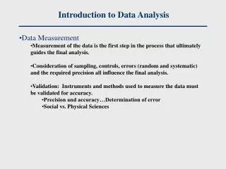
Introduction to Data Analysis • Data Measurement • Measurement of the data is the first step in the process that ultimately guides the final analysis. • Consideration of sampling, controls, errors (random and systematic) and the required precision all influence the final analysis. • Validation: Instruments and methods used to measure the data must be validated for accuracy. • Precision and accuracy…Determination of error • Social vs. Physical Sciences
Introduction to Data Analysis • Types of data • Univariate/Multivariate • Univariate: When we use one variable to describe a person, place, or thing. • Multivariate: When we use two or more variables to measure a person, place or thing. Variables may or may not be dependent on each other. • Cross-sectional data/Time-ordered data (business, social sciences) • Cross-Sectional: Measurements taken at one time period • Time-Ordered: Measurements taken over time in chronological sequence. • The type of data will dictate (in part) the appropriate data-analysis method.
Introduction to Data Analysis • Measurement Scales • Nominal or Categorical Scale • Classification of people, places, or things into categories (e.g. age ranges, colors, etc.). • Classifications must be mutually exclusive (every element should belong to one category with no ambiguity). • Weakest of the four scales. No category is greater than or less (better or worse) than the others. They are just different. • Ordinal or Ranking Scale • Classification of people, places, or things into a ranking such that the data is arranged into a meaningful order (e.g. poor, fair, good, excellent). • Qualitative classification only
Introduction to Data Analysis • Measurement Scales (business, social sciences) • Interval Scale • Data classified by ranking. • Quantitative classification (time, temperature, etc). • Zero point of scale is arbitrary (differences are meaningful). • Ratio Scale • Data classified as the ratio of two numbers. • Quantitative classification (height, weight, distance, etc). • Zero point of scale is real (data can be added, subtracted, multiplied, and divided).
Univariate Analysis/Descriptive Statistics • Descriptive Statistics • The Range • Min/Max • Average • Median • Mode • Variance • Standard Deviation • Histograms and Normal Distributions
Distributions Descriptive statistics are easier to interpret when graphically illustrated. However, charting each data element can lead to very busy and confusing charts that do not help interpret the data. Grouping the data elements into categories and charting the frequency within these categories yields a graphical illustration of how the data is distributed throughout its range. Univariate Analysis/Histograms
Univariate Analysis/Histograms With just a few columns this chart is difficult to interpret. It tells you very little about the data set. Even finding the Min and Max can be difficult. The data can be presented such that more statistical parameters can be estimated from the chart (average, standard deviation).
Univariate Analysis/Histograms • Frequency Table • The first step is to decide on the categories and group the data appropriately. (45, 49, 50, 53, 60, 62, 63, 65, 66, 67, 69, 71, 73, 74, 74, 78, 81, 85, 87, 100)
Univariate Analysis/Histograms • Histogram • A histogram is simply a column chart of the frequency table.
Histogram Univariate Analysis/Histograms Average (68.6) and Median (68) Mode (74) -1SD +1SD
Univariate Analysis/Normal Distributions • Distributions that can be described mathematically as Gaussian are also called Normal • The Bell curve • Symmetrical • Mean ≈ Median Mean, Median, Mode
Univariate Analysis/Skewed Distributions • When data are skewed, the mean and SD can be misleading • Skewness sk= 3(mean-median)/SD If sk>|1| then distribution is non-symetrical • Negatively skewed • Mean<Median • Sk is negative • Positively Skewed • Mean>Median • Sk is positive
Central Limit Theorem • Regardless of the shape of a distribution, the distribution of the sample mean based on samples of size N approaches a normal curve as N increases. • N must be less than the entire sample N=10
Univariate Analysis/Descriptive Statistics • The Range • Difference between minimum and maximum values in a data set • Larger range usually (but not always) indicates a large spread or deviation in the values of the data set. (73, 66, 69, 67, 49, 60, 81, 71, 78, 62, 53, 87, 74, 65, 74, 50, 85, 45, 63, 100)
Univariate Analysis/Descriptive Statistics • The Average (Mean) • Sum of all values divided by the number of values in the data set. • One measure of central location in the data set. Average = Average=(73+66+69+67+49+60+81+71+78+62+53+87+74+65+74+50+85+45+63+100)/20 = 68.6 Excel function: AVERAGE()
The data may or may not be symmetrical around its average value 0 2.5 7.5 10 4.8 0 2.5 7.5 10 4.8 Univariate Analysis/Descriptive Statistics
The Median The middle value in a sorted data set. Half the values are greater and half are less than the median. Another measure of central location in the data set. (45, 49, 50, 53, 60, 62, 63, 65, 66, 67, 69, 71, 73, 74, 74, 78, 81, 85, 87, 100) Median: 68 (1, 2, 4, 7, 8, 9, 9) Excel function: MEDIAN() Univariate Analysis/Descriptive Statistics
The Median May or may not be close to the mean. Combination of mean and median are used to define the skewness of a distribution. 0 2.5 7.5 10 6.25 Univariate Analysis/Descriptive Statistics
The Mode Most frequently occurring value. Another measure of central location in the data set. (45, 49, 50, 53, 60, 62, 63, 65, 66, 67, 69, 71, 73, 74, 74, 78, 81, 85, 87, 100) Mode: 74 Generally not all that meaningful unless a larger percentage of the values are the same number. Univariate Analysis/Descriptive Statistics
Univariate Analysis/Descriptive Statistics • Variance • One measure of dispersion (deviation from the mean) of a data set. The larger the variance, the greater is the average deviation of each datum from the average value. Variance = Average value of the data set Variance = [(45 – 68.6)2 + (49 – 68.6)2 + (50 – 68.6)2 + (53 – 68.6)2 + …]/20 = 181 Excel Functions: VARP(), VAR()
Standard Deviation Square root of the variance. Can be thought of as the average deviation from the mean of a data set. The magnitude of the number is more in line with the values in the data set. Univariate Analysis/Descriptive Statistics Standard Deviation = ([(45 – 68.6)2 + (49 – 68.6)2 + (50 – 68.6)2 + (53 – 68.6)2 + …]/20)1/2 = 13.5 Excel Functions: STDEVP(), STDEV()