Nondeterministic Automata vs Deterministic Automata

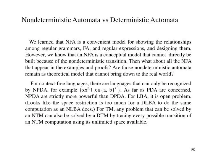
1. Nondeterministic Automata vs Deterministic Automata We learned that NFA is a convenient model for showing the relationships among regular grammars, FA, and regular expressions, and designing them. However, we know that an NFA is a conceptual model that cannot directly be built because of the nondeterministic transition. Then what about all the NFA that appear in the examples and proofs? Are those nondeterministic automata remain as theoretical model that cannot bring down to the real world? For context-free languages, there are languages that can only be recognized by NPDA, for example {xxR | x{a, b}* }. As far as PDA are concerned, NPDA are strictly more powerful than DPDA. For LBA, it is open problem. (Looks like the space restriction is too much for a DLBA to do the same computation as an NLBA does.) For TM, any problem that can be solved by an NTM can also be solved by a DTM by tracing every possible transition of an NTM computation using its unlimited space available.

2. a b {0,1,2} b a {1,2} b c a a b,c c 1 2 0 start start 0 c b,c {2} a,b,c c (a) An NFA (b) Converted DFA Fortunately, for NFA there is a straightforward way to transform them into DFA. (Actually it is based on the same idea that we used to eliminate -transitions.) The basic idea is to consider the set of states that can be reachable by a transition as a single state in deterministic transition. The following example will be enough to understand the technique. (We assume that the automaton has no -transitions.) Notice that the state with label {0, 1, 2} is from the set of states given by the nondeterministic transition (0, a) = {0, 1, 2}. Also notice that any state whose label contains an accepting state is defined as an accepting state in the deterministic machine.

3. b b q3 q1 q1 q34 a a a a b b q2 q2 q4 a b b Figure (a) Figure (b) Minimization Technique for DFA The number of states of an automaton has direct affect to the size of the machine realizing the automaton. Hence, it is very important to reduce the number of states, if possible. For PDA, LBA and TM, it is very difficult problem to reduce the number of states. However, for DFA there is very efficient algorithm for minimizing the number of states of a given DFA. Figure (a) below is a part of the state transition graph of a DFA M = ( Q ,  ,  , q0, F ), where  = { a, b }. Clearly, for every w   *, ( q3 , w ) is in an accepting state if and only if ( q4 , w )is. Hence, we can merge q3 and q4 into a single state as shown in Figure (b) without affecting the language of the machine.

4. a b 3 a a a 1 a b 3 b 0 4 a a, b b b 2 0 1,2 a b a, b 5 b a b 4,5 Figure (a) A DFA Figure (b) Reduced DFA State Reduction by Partitioning We say two states p and q are equivalent (or indistinguishable), if, for every string w   * , transition ( p, w )ends in an accepting state if and only if ( q, w) does. In the preceding slide states q3 andq4 are equivalent. There are efficient algorithms available for computing the sets of equivalent states of a given DFA. The following example shows a procedure using the set partitioning technique. The technique is similar to one that they use for partitioning people into groups (each having certain preferences) based on their responses to questionnaire. The following two slides show the detailed steps for computing equivalent state sets of the DFA in Figure (a) and constructing the reduced DFA shown in Figure (b).

5. State Reduction by Partitioning(cont’ed) • Step 0: Partition the states according to accepting/non-accepting. P1P2 { 3, 4, 5 } { 0, 1, 2 } Figure (a) Initial partition For a state q and symbol t, let Pi be the response of q on t , if (q, t) enters a state in Pi. • Step 1: Get the response of each state for each input symbol. Notice that States 3 and 0 show different responses from the ones of the other states in the same set. P1P2 p1 p1 p1 p2 p1 p1 a  a    {3, 4, 5 } {0, 1, 2 } b   b    p2 p1 p1 p2 p1 p1 Figure (b) Record responses for each input symbol

6. Step 2: Partition the sets according to the responses, and go to Step 1 until no partition occurs. • P11 P12 P21 P22 • p11 p11 p12 p12 • a a   • {4, 5} {3} {1, 2} {0} • b  b   • p11 p11 p11 p11 • Figure (c) Partition the set, and record responses for each input symbol • No further partition is possible for the sets P11and P21. So the final partition results areas follows. • {4, 5} {3} {1, 2} {0} • (d) Final partition