
CSI5388 Model Selection
E N D
Presentation Transcript
CSI5388Model Selection Based on “Key Concepts in Model Selection: Performance and Generalizability” by Malcom R. Forster
What is Model Selection? • Model Selection refers to the process of optimizing a model (e.g., a classifier, a regression analyzer, and so on). • Model Selection encompasses both the selection of a model (e.g., C4.5 versus Naïve Bayes) and the adjustment of a particular model’s parameters (e.g., adjusting the number of hidden units in a neural network).
What are potential issues with Model Selection? • It is usually possible to improve a model’s fit with the data (up to a certain point). (e.g., more hidden units will allow a neural network to fit the data on which it is trained, better). • The question is, however, where should the distinction between improving the model and hurting its performance on novel data (overfitting) be drawn? • We want the model to use enough information from the data set to be as unbiased as possible, but we want it to discard all the information it needs to make it generalize as well as it can (i.e., fare as well as possible on a variety of different context). • As such, model selection is very tightly linked with the issue of the Bias/Variance tradeoff.
Why is the issue of Model Selection considered in a course on evaluation? • By evaluation, in this course, we are principally concerned with the issue of evaluating a classifier once its tuning is finalized. • However, we must keep in mind that evaluation has a broader meaning in the sense that while classifiers are being chosen and tuned, another evaluation (not final) must take place to make sure that we are on the right track. • In fact, there is a view that does not distinguish between the two aspects of evaluation above, but rather, assumes that the final evaluation is nothing but a continuation of the model selection process.
Different Approaches to Model Selection • We will survey different approaches to Model Selection not all of them most useful to our problem of maximizing predictive performance. • In particular, we will consider: • The Method of Maximum Likelihood • Classical Hypothesis Testing • Akaike’s Information Criterion • Cross-Validation Techniques • Bayes Method • Minimum Description Length
The Method of Maximum Likelihood (ML) • Out of the Maximum Likelihood (ML) hypotheses in the competing models, select the one that has the greatest likelihood or log-likelihood. • This method is the antithesis of Occam’s razor as, in the case of nested models, it can never favour anything less than the most complex of all competing models.
Classical Hypothesis Testing I • We consider the comparison of nested models, in which we decide to add or omit a single parameter θ. So we are choosing between hypotheses θ=0 and θ ≠0. • θ=0 is considered the null hypothesis. • We set up a 5% critical region such that if θ^, the maximum likelihood (ML) estimate for θ, is sufficiently close to 0, then the null hypothesis is not rejected (p< 0.5, two tailed). • Note that when the test fails to reject the null hypothesis, it is favouring the simpler hypothesis in spite of its poorer fit (because θ^ fits better than θ=0), if the null hypothesis is the simpler of the two models. • So classical hypothesis testing succeeds in trading off goodness-of-fit for simplicity.
Classical Hypothesis Testing II • Question: Since classical hypothesis testing succeeds in trading off goodness-of-fit for simplicity, why do we need any other method for model selection? • That’s because it doesn’t apply well to non-nested models (when the issue is not one of adding or not a parameter. • In fact, classical hypothesis testing works on some model selection problems only by chance: it was not purposely designed to work on them.
Akaike’s Information Criterion I • Akaike’s Information Criterion (AIC) minimizes the Kullback-Leibler distance of the selected density from the true density. • In other words, the AIC rule maximizes log f(x; θ= θ^)/n – k/n [where n is the number of observed data, k is the number of adjustable parameters and f(x, θ) is the density]. • The first term in the formula above measures fit per datum, while the second term penalizes complex models. • AIC without the second term would be the same as Maximum Likelihood (ML).
Akaike’s Information Criterion II • What is the difference between AIC and classical hypothesis testing? • AIC applies to nested and non-nested models. All that’s needed for AIC is the ML values of the models, and their k and n values. There is no need to choose a null hypothesis. • AIC effectively tradeoffs Type I or Type II error. As a result, AIC may give less weight to simplicity than to fit than classical hypothesis testing.
Cross-Validation Techniques I • Use a calibration set (training set) and a test set to determine the best model. • Note, however, that the test set cannot be the same as the test set we are used to, so in fact, we need three sets: training, validation and test. • This because the training set is different from the training and validation sets taken together (our goal is to optimize the model on that set), it is best to use leave-one-out on training+validation to select a model. • This is because training + validation – one data point is closer to training + validation than training, alone.
Cross-Validation Techniques II • Although cross-validation techniques makes no appeal to simplicity whatsoever, it is asymptotically equivqlent to AIC. • This is because minimizing Kullback-Liebler distance between the ML density is the same as maximizing predictive accuracy if that is defined in terms of the expected log-likelihood of new data generated by the true density (Forster and Sober, 1994). • More simply, I guess that this can be explained by the fact that there is truth to Occam’s razor: the simpler models are the best at predicting the future, so by optimizing predictive accuracy, we are unwittingly trading off goodness-of-fit with model simplicity.
Bayes Method I • Bayes method says that models should be compared by their posterior probabilities. • Schwartz 1978 assumed that the prior probabilities of all models were equal, and then derived an asymptotic expression for the likelihood of a model as follows: • A model can be viewed as a big disjunction which asserts that either the first density in the set is the true density, or the second, the third and so on. • By the probability calculus, the likelihood of a model is, therefore, the average likelihood of its members where each likelihood is weighed by the prior probability of the particular density given that the model is true. • In other words, the Bayesian Information Criterion (BIC) rule is to favour the model with the highest value of log f(x; θ= θ^)/n – [log(n)/2]k/n • Note: The Bayes method and BIC criterion are not always the same thing.
Bayes Method II • There is a philosophical disagreement between the Bayesian school and other researchers. • The Bayesians assume that BIC is an approximation of the Bayesian method, but this is the case only if the models are quasi-nested. If they are truly nested, there is no implementation of Occam’s razor whatsoever. • Bayes method and AIC optimize entirely different things and this is why they don’t always agree.
Minimum Description Length Criteria • In Computer Science, the best known implementation of Occam’s razor is the minimum description length criteria (MDL) or the minimum message length criteria (MML). • The motivating idea is that the best model is one that facilitates the shortest encoding of observed data. • Among the various implementations of MML and MDL one is asymptoically equivalent to BIC.
Limitation of the different approaches to Model Selection I • One issue with all these model selection methods is called: Selection bias, and can’t be easily corrected. • Selection bias corresponds to the fact that model criteria are particularly risky when a selection is made from a large number of competing models. • The random fluctuation in the data will increase the scores of some models more than others. The more models there are, the greater the chance that the winner won by luck rather than by merit.
Limitation of the different approaches to Model Selection II • The Bayesian method is not as sensitive to the problem of selection bias because its predictive density is a weighted average of all the densities in all domains. However, this advantage comes at the expense of making the prediction rather imprecise. • To defray problems of Selection Bias Golden, 2000 suggests a three-way statistical test that includes: accept, reject, or suspend judgement. • Browne, 2000 emphasizes that selection criteria should not be followed blindly. He warns that the term ‘selection’ suggests something definite, which in fact has not been reached.
Limitation of the different approaches to Model Selection III • If model selection is seen as using data sampled from one distribution in order to predict data sampled from another, then the methods previously discussed will not work well, since they assume that the two distributions are the same. • In this case, errors of estimation do not arise solely from small sample fluctuations, but also from the failure of the sampled data to properly represent the domain of prediction. • We will now discuss a method by Busemeyer and Wang 2000 that deals with this issue of extrapolation or generalization to new data.
Model Selection for New Data [Busemeyer and Wang 2000 ] • One response to the fact that if extrapolation to new data does not work is: “there is nothing we can do about that”. • Busemeyer and Wang (2000) as well as Forster do not share this conviction. Instead, they designed the generalization criterion methodology which state that successful extrapolation in the past may be a useful indicator of further extrapolation. • The idea is to find out whether there are situations in which past extrapolation is a useful indicator of future extrapolation, and whether this empirical information is not already exploited by the standard selection criteria.
Experimental Results I • Forster ran some experiments to test this idea. • He found that on the task of fitting data coming from the same distribution, the model selection methods we discussed were adequate at predicting the best models: the most complex models were always the better ones (we are in a situation where a lot of data is available to model the domain, and, thus, the fear of overfitting in case of a complex model is not present). • On the task of extrapolating from one domain to the next, the model selection methods were npt adequate since they didn’t reflect the fact that the best classifier were not necessarily the most complex ones.
Experimental Results II • The generalization methodology divides the training set into two subdomains, but the subdomains are chosen so that the direction of the test extrapolation is most likely to indicate the success of the wider extrapolation. • This approach seems to yield better results than that of standard model selection. • For a practical example of this kind of approach, see Henchiri & Japkowicz, 2007.
Experimental Results III • Overall, it does appear that the generalization scores provide us with useful empirical information that is not exploited by the standard selection criteria. • There are some cases, where the information is not only unexploited, but it is also relatively clear cut and decisive. • Such information might at least supplement the standard criteria