Week 2 Basics of MD Simulations
610 likes | 796 Vues
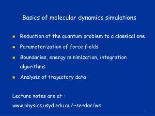
Week 2 Basics of MD Simulations Lecture 3: Force fields (empirical potential functions among atoms) Boundaries and computation of long-range interactions

Week 2 Basics of MD Simulations
E N D
Presentation Transcript
Week 2 • Basics of MD Simulations • Lecture 3: Force fields (empirical potential functions among atoms) Boundaries and computation of long-range interactions • Lecture 4: Molecular mechanics (T=0, energy minimization) MD simulations (integration algorithms, constrained dynamics, ensembles)
Empirical force fields (potential functions) Problem: Reduce the ab initio potential energy surface among the atoms To a classical many-body interaction in the form Such a program has been tried for water but so far it has failed to produce a classical potential that works. In strongly interacting systems, it is difficult to describe the collective effects by summing up the many-body terms. Practical solution: Truncate the series at the two-body level and assume (hope!) that the effects of higher order terms can be absorbed in U2 by reparametrizing it.
Non-bonded interactions Interaction of two atoms at a distance R can be decomposed into 4 pieces • Coulomb potential (1/R) • Induced polarization (1/R2) • Dispersion (van der Waals) (1/R6) • Short range repulsion (e-R/a) The first two can be described using classical electromagnetism 1. Coulomb potential: 2. Induced polarization: Dipole field Total polarization int. (Initial and final E fields in iteration)
The last two interactions are quantum mechanical in origin. Dispersion is a dipole-dipole interaction that arises from quantum fluctuations (electronic excitations to non-spherical states) Short range repulsion arises from Pauli exclusion principle (electron clouds of two atoms avoid each other), so it is proportional to the electron density The two interactions are combined using a 12-6 Lennard-Jones (LJ) potential Here e corresponds to the depth of the potential at the minimum; 21/6σ Combination rules for different atoms:
Because the polarization interaction is many-body and requires iterations, it has been neglected in most force fields. The non-bonded interactions are thus represented by the Coulomb and 12-6 LJ potentials. Popular water models (rigid) Model RO-H (Å) qHOH qH (e) e (kT) s (Å) m (D) k (T=298 C) SPC 1.0 109.5 0.410 0.262 3.166 2.27 65±5 TIP3P 0.957 104.5 0.417 0.257 3.151 2.35 97±7 Exp. Gas 1.86 80 Ab initio Water 3.00 SPC: simple point charge TIP3P: transferable intermolecular potential with 3 points
There are hundreds of water models in the market, some explicitly including polarization interaction. But as yet there is no model that can describe all the properties of water successfully. SPC and TIP3P have been quite successful in simulation of biomolecules, and have become industry standards. However, the mean field description of the polarization interaction is bound to break in certain situations: • Ion channels, cavities • Interfaces • Divalent ions To deal with these, we need polarizable force fields. Grafting point polarizabilities on atoms and fitting the model to data has not worked well. Ab initio methods are needed to make further progress.
Covalent bonds In molecules, atoms are bonded together with covalent bonds, which arise from sharing of electrons in partially occupied orbitals. In order to account for the dipole moment of a molecule in a classical representation, partial charges are assigned to the atoms. If the bonds are very strong, the molecule can be treated as rigid as in water molecule. In most large molecules, however, the structure is quite flexible and this must be taken into account for a proper description of the molecules. This is literally done by replacing the bonds by springs. The nearest neighbour interactions involving 2, 3 and 4 atoms are described by harmonic and periodic potentials bond stretching bending torsion (not very good)
Interaction of two H atoms in the ground (1s) state can be described using Linear Combinations of Atomic Orbitals (LCAO) From symmetry, two solutions with lowest and highest energies are: + Symmetric - Anti-symmetric
The R dependence of the potential energy is approximately given by the Morse potential Where De: dissociation energy Re: equilibrium bond distance controls the width of the potential Classical representation: k
Electronic wave functions for the 1s, 2s and 2p states in H atom H2 molecule:
In carbon, 4 electrons (in 2s and 2p) occupy 4 hybridized sp3 orbitals Tetrahedral structure of sp3 Thus carbon needs 4 bonds to have a stable configuration. Nitrogen has an extra electron, so needs 3 bonds. Oxygen has 2 extra electrons, so needs 2 bonds.
For a complete description of flexibility, we need, besides bond stretching, bending and torsion. The former can be described with a harmonic form: While the latter is represented with a periodic function Bond stretching and bending interactions are quite strong and well determined from spectroscopy. Torsion is much weaker compared to the other two and is not as well determined. Following QM calculations, they have been revamped recently (e.g., CMAP corrections in the CHARMM force field), which resulted in a better description of proteins.
An in-depth look at the force fields Three force fields, constructed in the eighties, have come to dominate the MD simulations • CHARMM (Karplus @ Harvard) Optimized for proteins, works well also for lipids and nucleic acids • AMBER (Kollman & Case @ UCSF) Optimized for nucleic acids, otherwise quite similar to CHARMM 3. GROMOS (Berendsen & van Gunsteren @ Groningen) Initially optimized for lipids and did not work very well for proteins (smaller partial charges in the carbonyl and amide groups) but it has been corrected in the more recent versions. The first two use the TIP3P water model and the last one, SPC model. They all ignore the polarization interaction. Polarizable versions have been under construction for over a decade but no working code yet.
Charm parameters for alanine Partial charge (e) ATOM N -0.47 |ATOM HN 0.31 HN—NATOM CA 0.07 | HB1ATOM HA 0.09 | /GROUP HA—CA—CB—HB2ATOM CB -0.27 | \ATOM HB1 0.09 | HB3ATOM HB2 0.09 O=CATOM HB3 0.09 |ATOM C 0.51ATOM O -0.51Total charge: 0.00
Bond lengths : kr (kcal/mol/Å2) r0 (Å)N CA 320. 1.430 (1)CA C 250. 1.490 (2)C N 370. 1.345 (2) (peptide bond) O C 620. 1.230 (2) (double bond)N H 440. 0.997 (2)HA CA 330. 1.080 (2)CB CA 222. 1.538 (3)HB CB 322. 1.111 (3) • NMA (N methyl acetamide) vibrational spectra • Alanine dipeptide ab initio calculations • From alkanes
Bond angles : kq (kcal/mol/rad2) q0 (deg)C N CA 50. 120. (1)C N H 34. 123. (1)H N CA 35. 117. (1)N CA C 50. 107. (2)N CA CB 70. 113.5 (2)N CA HA 48. 108. (2)HA CA CB 35. 111. (2)HA CA C 50. 109.5 (2)CB CA C 52. 108. (2)N C CA 80. 116.5 (1)O C CA 80. 121. (2)O C N 80. 122.5 (1) Total 360 deg. Total 360 deg.
Dihedrals: Basic dihedral configurations trans cis Definition of the dihedral angle for 4 atoms A-B-C-D
Dihedral parameters: Vn (kcal/mol) n f0 (deg) Name C N CA C 0.2 1 180. f N CA C N 0.6 1 0. y CA C N CA 1.6 1 0. w H N CA CB 0.0 1 0. H N CA HA 0.0 1 0. C N CA CB 1.8 1 0. CA C N H 2.5 2 180. O C N H 2.5 2 180. O C N CA 2.5 2 180.
(Sasisekharan) a-helix • ~ -57o • ~ -47o
When one of the 4 atoms is not in a chain (e.g. O bond with C in CA-C-N), then an improper dihedral interaction is used to constrain that atom. Most of the time, off-the-chain atom is constrained to a plane using: CA C O N Where q is the angle C=O bond makes with the CA-C-N plane, and q0 = 180 which enforces a planar configuration.
Boundaries In macroscopic systems, the effect of boundaries on the dynamics of biomolecules is minimal. In MD simulations, however, the system size is much smaller and one has to worry about the boundary effects. • Using nothing (vacuum) is not realistic for bulk simulations. • Minimum requirement: water beyond the simulation box must be treated using a continuum representation (reaction field). An intermediate zone is treated using stochastic boundary conditions. • Most common solution: periodic boundary conditions. The simulation box is replicated in all directions just like in a crystal. The cube and rectangular prism are the obvious choices for a box shape, though there are other shapes that can fill the space (e.g. hexagonal prism and rhombic dodecahedron).
Periodic boundary conditions in two dimensions: 8 nearest neighbours Particles in the box freely move to the next box, which means they appear from the opposite side of the same box. In 3-D, there are 26 nearest neighbours.
Treatment of long-range interactions Problem: the number of non-bonded interactions grows as N2 where N is the number of particles. This is the main computational bottle neck that limits the system size. A simple way to deal with this problem is to introduce a cutoff radius for pairwise interactions (together with a switching function), and calculate the potential only for those within the cutoff sphere. This is further facilitated by creating non-bonded pair lists, which are updated every 10-20 steps. • For Lennard-Jones (6-12) interaction, which is weak and falls rapidly, this works fine and is adapted in all MD codes. • Coulomb interaction, however, is very strong and falls very slowly. [Recall the Coulomb potential between two unit charges, U=560 kT/r (Å)] Hence use of any cutoff is problematic and should be avoided.
This problem has been solved by introducing the Ewald sum method. All the modern MD codes use the Ewald sum method to treat the long-range interactions without cutoffs. Here one replaces the point charges with Gaussian distributions, which leads to a much faster convergence of the sum in the reciprocal (Fourier) space. The remaining part (point particle – Gaussian) falls exponentially in real space, hence can be computed easily using a cutoff radius (~10 Å). The mathematical details of the Ewald sum method is given in the following appendix. Please read it to understand how it works in practice.
Appendix: Ewald summation method The coulomb energy of N charged particles in a box of volume V=LxLyLz Here with integer values for n. The prime on the sum signifies that i=j is not included for n=0. Ewald’s observation (1921): in calculating the Coulomb energy of ionic crystals, replacing the point charges with Gaussian distributions leads to a much faster convergence of the sum in the reciprocal (Fourier) space. The remaining part (point particle – Gaussian) falls exponentially in real space, hence can be computed easily.
The Poisson equation and it’s solution: For a point charge q at the origin: When the charge q has a Gaussian distribution:
This result is obtained most easily by integrating the Poisson equation Integrate 0 to r :
Writing the charge density as For the second part, the potential due to a charge qj at rj is given by: Where erfc(x) is the complementary error function which falls as Thus choosing 1/ about an Angstrom, this potential converges quickly. Typically, it is evaluated using a cutoff radius of ~10 Å, so the original box with N particles is sufficient for this purpose (with the nearest image convention). The direct (short-range) part of the energy of the system is:
The Gaussian part converges faster in the reciprocal (Fourier) space hence best evaluated as a Fourier series The Poisson equation in the Fourier space For a point charge q at the origin:
When the charge q has a Gaussian distribution: Multiply each integral by to compete the square Each Gaussian integral then gives The corresponding potential in the Fourier space
The Gaussian charge density for the periodic box Which yields for the potential
Transforming back to the real space The reciprocal space (long-range) part of the system’s energy:
This energy includes the self-energy of the Gaussian density which needs to be removed So the total energy is:
Molecular mechanics Molecular mechanics deals with the static features of biomolecular systems at T=0 K, that is, particles do not have any kinetic energy. [Note that in molecular dynamics simulations, particles have an average kinetic energy of (3/2)kT, which is substantial at room temp., T=300 K] Thus the energy is given solely by the potential energy of the system. Two important applications of molecular mechanics are: • Energy minimization (geometry optimization): Find the coordinates for the configuration that minimizes the potential energy (local or absolute minimum). • Normal mode analysis: Find the vibrational excitations of the system built on the absolute minimum using the harmonic approximation.
Energy minimization The initial configuration of a biomolecule whether experimentally determined or otherwise does not usually correspond to the minimum of the potential energy function. It may have large strains in the backbone that would take a long time to equilibrate in MD simulations, or worse, it may have bad contacts (i.e. overlapping van der Waals radii), which would crash the MD simulation in the first step! To avoid such mishaps, it is a standard practice to minimize the energy before starting MD simulations. Three popular methods for analytical forms: • Steepest descent (first derivative) • Conjugate gradient (first derivative) • Newton-Raphson (second derivative)
Steepest descent: Follows the gradient of the potential energy function U(r1, …,rN) at each step of the iteration where iis the step size. The step size can be adjusted until the minimum of the energy along the line is found. If this is expensive, a single step is used in each iteration, whose size is adjusted for faster convergence. • Works best when the gradient is large (far from a minimum), but tends to have poor convergence as a minimum is approached because the gradient becomes smaller. • Successive steps are always mutually perpendicular, which can lead to oscillations and backtracking.
A simple illustration of steepest descent with a fixed step size in a 2D energy surface (contour plots)
Conjugate gradient: Similar to steepest descent but the gradients calculated from previous steps are used to help reduce oscillations and backtracking (For the first step, d is set to zero) • Generally one finds a minimum in fewer steps than steepest descent, e.g. it takes 2 steps for the 2D quadratic function, and ~n steps for nD. • But conjugate gradient may have problems when the initial conformation is far from a minimum in a complex energy surface. • Thus a better strategy is to start with steepest descent and switch to conjugate gradient near the minimum.
Newton-Raphson: Requires the second derivatives (Hessian) besides the first. Predicts the location of a minimum, and heads in that direction. To see how it works in a simple situation, consider the quadratic 1D case In general For a quadratic energy surface, this method will find the minimum in one step starting from any configuration.
Construction and inversion of the 3Nx3N Hessian matrix is computationally demanding for large systems (N>100). • It will find a minimum in fewer steps than the gradient-only methods in the vicinity of the minimum. • But it may encounter serious problems when the initial conformation is far from a minimum. • A good strategy is to start with steepest descent and then switch to alternate methods as the calculations progress, so that each algorithm operates in the regime for which it was designed. Using the above methods, one can only find a local minimum. To search for an absolute minimum, Monte Carlo methods are more suitable. Alternatively, one can heat the system in MD simulations, which will facilitate transitions to other minima.
Normal mode analysis Assume that the minimum energy of the system is given by the 3N coordinates, {r0i}. Expanding the potential energy around the equilibrium configuration gives Ignoring the constant energy, the leading term is that of a system of coupled harmonic oscillators. In a normal mode, all the particles in the system oscillate with the same frequency w. To find the normal modes, first express the 3N coordinates as {xi, i=1,…,3N}.
The potential energy becomes where the spring constants are given by the Hessian as Introducing the 3Nx3N diagonal mass matrix M The secular equation for the normal modes is given by
For a 3Nx3N matrix, solution of the secular equation will yield 3N eigenvalues, wi and the corresponding eigenvectors, ai Of these, 3 correspond to translations and 3 to rotations of the system. Thus there are 3N-6 intrinsic vibrational modes of the system. At a given temperature T, the motion of the i’th coordinate is given by The mean square displacement of the coordinates and atoms:
A simple example: normal modes of water molecule Water molecule has 9-6=3 intrinsic vibrations, which correspond to symmetric and anti-symmetric stretching of H atoms and bending. Because of H-bonding, water molecules in water cannot freely rotate but rather librate (wag or twist). Wave numbers: 3652 cm-1 3756 cm-1 1595 cm-1 (200 cm-1~1 kT) Excitation energies >> kT, which justifies the use of a rigid model for water.
Normal modes of a small protein BPTI (Bovine pancreatic tyripsin inhibitor) Some characteristic frequencies (in cm-1) Stretching Bending Torsion H-N: 3400-3500 H-C-H: 1500 C=C: 1000 H-C: 2900-3000 H-N-H: 1500 C-O: 300-600 C=C, C=O: 1700-1800 C-C=O: 500 C-C: 300 C-C, C-N: 1000-1250 S-S-C: 300 C-S: 200
Applications to domain motions of proteins • Many functional proteins have two main configurations called, for example, resting & excited states, or open & closed states. • Proteins can be crystallized in one of these states – the other configuration need to be found by other means. • The configurational changes that connect these two states usually involve large domain motions that could take milli to micro seconds, which is outside the reach of current MD simulations. • Normal mode analysis can be used to identify such collective motions in proteins and predict the missing state that is crucial for description of the protein function. • Examples: 1. Gating of ion channels (open & closed states) 2. Opening and closing of gates in transporters
Molecular dynamics In MD simulations, one follows the trajectories of N particles according to Newton’s equation of motion: where U(r1,…, rN) is the potential energy function consisting of bonded and non-bonded interactions (Coulomb and LJ 6-12). We have already discussed force fields and boundary conditions in some detail. Here, we will consider: • Integration algorithms, e.g., Verlet, Leap-frog • Initial conditions and choice of the time step • Constrained dynamics for rigid molecules (SHAKE and RATTLE) • MD simulations at constant temperature and pressure
Integration algorithms Given the position and velocities of N particles at time t, a straightforward integration of Newton’s equation of motion yields at t+Dt (1) (2) In practice, variations of these equations are implemented in MD codes In the popular Verlet algorithm, one eliminates velocities using the positions at t-Dt, Adding with eq. (2), yields: