Choice modelling - an example
This study explores the market dynamics surrounding Perfect Cheese, focusing on processed cheese and natural cheddar offerings. It aims to assess market sensitivity to price, market share potential, and cannibalization effects following the launch of Perfect Cheese. By employing Discrete Choice Modelling, we evaluate consumer acceptance, pricing impacts pre-and post-trial, and sensory performance against competitors. The findings support effective brand positioning and inform strategic pricing decisions to enhance market performance.


Choice modelling - an example
E N D
Presentation Transcript
Background • Bonlac changing processed cheese and natural cheddar offering from Bega to Perfect Cheese • Previous research has: • Explored an appropriate positioning for Perfect Cheese • Identified the optimal pack design • Further research is required to: • Understand market response to the new range of Perfect Cheese in terms of: • Price sensitivity • Market share potential • Cannibalisation effects • In addition, feedback on sensory performance of Perfect Cheese products relative to competitors, in order to support positioning platform ( not discussed today)
Pricing Objectives • To understand the impact of launching of Perfect in the Processed Cheese and Light Cheddar Block markets • Understanding initial impact (pre-trial) • Understand longer term impact (post-trial) • Understand the price sensitivity of each user group
Sensory Objectives • To evaluate the Perfect cheese slice and block products relative to competitive offerings in terms of: • Acceptability (unbranded vs branded) • Sensory profiles • Relative to consumer ideals • Purchase intentions • Ability to support brand positioning expectations
Pre-trial Discrete Choice Modelling Sensory Evaluation 1. All products unbranded 2. Perfect Cheese product branded Post-trial Discrete Choice Modelling Method • Central location test at Takapuna
Sample Population • N=30 each of: • Light Slice users • Super Light Slice users • Cheddar Slice users • Reduced Fat Cheddar Block users • Sample population: • Females MHS, 20-65 years • Mix of household types (mainly families with kids)
Pricing Methodology • 15 shelves - pre/post presented to each of 30 people in 4 user groups • Light Slices • Super Light Slices • Cheddar Slices • Light Cheddar Block • In each shelf range of prices consumers get to choose only one • Imitates shopping experience • Idealised situations (100% awareness of Perfect) • House-brands included
Whoa there! - How did we get to this conclusion? • 3 brands of interest – Mainland/Chesdale and Perfect • The other 2, Pams and First Choice area at fixed, lower prices, prices • Decided to go with 3 price (low $1.99/medium $2.29 /high $2.59) points/brand • Why? • Therefore we have 33 =27 possible combinations • Decided to choose a sample of 15 to reduce respondent fatigue and to ensure we could measure all 2 order interaction effects • eg: does a high price of Chesdale result in different pricing response for Perfect than if it were a low price • This phenomenon is quite common so needs to be taken into account
The design Discuss:
Some points • Note that we have decided to mode/post data together • Not how the data is agrregated now • Compare this to what we have: Preprice 1 Cumulative Cumulative PRE1 Frequency Percent Frequency Percent ƒƒƒƒƒƒƒƒƒƒƒƒƒƒƒƒƒƒƒƒƒƒƒƒƒƒƒƒƒƒƒƒƒƒƒƒƒƒƒƒƒƒƒƒƒƒƒƒƒƒƒƒƒƒƒƒƒ 1 8 26.67 8 26.67 2 7 23.33 15 50.00 3 1 3.33 16 53.33 4 12 40.00 28 93.33 5 2 6.67 30 100.00 Preprice 2 Cumulative Cumulative PRE2 Frequency Percent Frequency Percent ƒƒƒƒƒƒƒƒƒƒƒƒƒƒƒƒƒƒƒƒƒƒƒƒƒƒƒƒƒƒƒƒƒƒƒƒƒƒƒƒƒƒƒƒƒƒƒƒƒƒƒƒƒƒƒƒƒ 1 28 93.33 28 93.33 2 1 3.33 29 96.67 4 1 3.33 30 100.00 Preprice 3 Cumulative Cumulative PRE3 Frequency Percent Frequency Percent ƒƒƒƒƒƒƒƒƒƒƒƒƒƒƒƒƒƒƒƒƒƒƒƒƒƒƒƒƒƒƒƒƒƒƒƒƒƒƒƒƒƒƒƒƒƒƒƒƒƒƒƒƒƒƒƒƒ 1 4 13.33 4 13.33 2 3 10.00 7 23.33 3 15 50.00 22 73.33 4 6 20.00 28 93.33 5 2 6.67 30 100.00
Some Points … • The variable T denote 1= choice, 2 = no choice • The resulting ‘doubling up” of all rows • The variable SET represents the appropriate scenario • For each scenario there are 10 =5*2 rows • Variables like CSD_MLD represents Chesdale’s effect on Mainland and so is in the relevant rows for Mainland but is Chesdale’s price • Remind me to give you a Splus function called SAS.DCM.FORMAT that helps format the appropriate design matrix for this data
Some more code data temp; set hold.cslmodel; PR_Mld2 = PR_Mld**2; PR_Prf2 = PR_Prf**2; PR_Anc2 = PR_Anc**2; PR_FC2 = PR_FC**2; PR_Pam2 = PR_Pam**2; DMld = POST*Mld; DPrf = POST*Prf; DAnc = POST*Anc; Dpam = POST*pam; Dfc = POST*FC; DPR_Mld = POST*PR_Mld; DPR_Prf = POST*PR_Prf; DPR_Anc = POST*PR_Anc; DPR_Pam = POST*PR_Pam; DPR_FC = POST*PR_FC; . . . DPam_Prf =POST*Pam_Prf; Note: coding up the pre/post effects DPam_Anc =POST*Pam_Anc; and quadraticprice effects DPam_FC =POST*Pam_FC ; run;
Analysing the data Saving this data: data hold.cslmodel; set temp; run; Now we are ready to start finding the correct model: ** trial and error to obtain the ‘correct’ model proc phreg data =hold.cslmodel outest =betas nosummary; strata set; model t*t(2) = CsD Mld Prf FC Pam PR_CsD PR_Mld PR_Prf PR_FC PR_pam PR_CsD2 PR_Mld2 PR_FC2 PR_pam2 DCsD DMld DPrf Dpam Dfc DPR_CsD DPR_Mld DPR_Prf DPR_FC DPR_Pam DPR_CsD2 DPR_Mld2 DPR_Prf2 DPR_FC2 DPR_pam2 DCsD_Mld DCsD_Prf DCsD_FC DCsD_Pam DMld_CsD DMld_Prf DMld_FC DMld_Pam DPrf_CsD DPrf_Mld DPrf_FC DPrf_Pam DFC_CsD DFC_Mld DFC_Prf DFC_Pam DPam_CsD DPam_Mld DPam_Prf DPam_FC /ties =breslow; freq freq; run;
Analysing the data… • The final model: procphregdata =hold.cslmodel outest =betas nosummary; strata set; model t*t(2) = CsD Mld Prf FC Pam PR_CsD PR_Mld PR_Prf PR_FC PR_pam PR_CsD2 PR_Mld2 PR_FC2 PR_pam2 DPrf DCsD_Prf /ties =breslow; freq freq; run;
Analysing the data… • Output: Analysis of Maximum Likelihood Estimates Parameter Standard Hazard Variable DF Estimate Error Chi-Square Pr > ChiSq Ratio CSD 1 62.03446 10.46407 35.1451 <.0001 8.734E26 MLD 1 53.51747 11.68024 20.9936 <.0001 1.747E23 PRF 1 12.41570 1.09299 129.0359 <.0001 246643.1 FC 1 1.15688 0.16214 50.9094 <.0001 3.180 PAM 0 0 . . . . PR_CSD 1 -48.72340 9.27818 27.5772 <.0001 0.000 PR_MLD 1 -41.00351 10.42944 15.4568 <.0001 0.000 PR_PRF 1 -5.23230 0.49984 109.5801 <.0001 0.005 PR_FC 0 0 . . . . PR_PAM 0 0 . . . . PR_CSD2 1 9.65004 2.03784 22.4241 <.0001 15522.40 PR_MLD2 1 7.85671 2.30708 11.5972 0.0007 2583.017 PR_FC2 0 0 . . . . PR_PAM2 0 0 . . . . DPRF 1 2.78607 1.13648 6.0098 0.0142 16.217 DCSD_PRF 1 -0.88705 0.48077 3.4042 0.0650 0.412