Nearcasting Convection using GOES Sounder Data
1k likes | 1.11k Vues
Utilizing GOES Sounder data to improve nearcasting for severe weather outbreaks, filling the gap between radar nowcasts and NWP models. Reduces loss of life and property damage, provides valuable weather information for better decision-making.

Nearcasting Convection using GOES Sounder Data
E N D
Presentation Transcript
Nearcasting Convection using GOES Sounder Data ROBERT M. AUNE AND RALPH PETERSENNOAA/ASPB/STARJORDAN GERTH AND SCOTT LINDSTROMSSEC / CIMSS
Requirement, Science, and Benefit Requirement/Objective Mission Goal: Weather and water Increase lead time and accuracy for weather and water warnings and forecasts Improve predictability of the onset, duration, and impact of hazardous and severe weather and water events Increase development, application, and transition of advanced science and technology to operations and services Science Can observations from a geostationary IR sounder be used to predict severe weather outbreaks 1 to 6 hours in advance, filling the gap between radar nowcasts and NWP models? Benefits Reduce loss of life, injury and damage to the economy Better, quicker, and more valuable weather and water information to support improved decisions Increased customer satisfaction with weather and water information and services
Nearcasting uses GOES Sounder Data • The GOES Sounder includes three separate water vapor channels • The water vapor channels have weighting functions that peak in different parts of the troposphere (longer wavelengths see farther down into the atmosphere) • Therefore have a three-dimensional look at atmospheric moisture
Note how sounder yields data at three levels! http://cimss.ssec.wisc.edu/goes/wf/faq.html
Note that the peak in the weighting function descends as the sounding dries out – you are looking at the radiation emitted by water vapor. As the sounding dries, less water vapor aloft to emit, so the sensor ‘sees’ farther down into the atmosphere (compare this page with the previous page)
Imager Water Vapor for weighting function slides Note Brightness Temperature values at CHS and LBF
Imager Water Vapor for weighting function slides Imager Water Vapor for weighting function slides Note Brightness Temperature values at CHS and LBF
Nearcasting uses GOES Sounder Data • Retrievalstransform observed Sounder radiances to more common meteorological variables (e.g. temperature, dewpoint) that can then be used to compute other variables (e.g. Lifted Index, CAPE) • Retrievals require clear skies • Is there a way to ‘move’ the clear pixels now to future positions that may be cloudy?
Nearcasting Severe Convection Using the GOES Sounder GOES sounder provides hourly snapshots of layer-averaged stability parameters (for example, Qe). These observations can be assimilated at multiple levels into a Lagrangian model to provide fast, short-term projections of atmospheric stability. Lagrangian model uses model winds (u,v) and geopotential heights to guide motion of observations. Model output and sounder retrievals are blended together to yield t = 0 observations – thus, there is more horizontal coverage at t = 0 than just from sounder retrievals alone (cloudy regions and eclipse regions can be included)
Premise: Sounder gives information on distinct layers in atmosphere at observation time Winds from a numerical model can move those slabs of moisture around Question: Where does Convective Instability develop because of the moving slabs? Very Dry Layer Somewhat Moist Layer Very Moist Layer
Observations at this time are limited over the East Coast by plenty of cloudiness
00-h fields include information from previous runs; areal extent of information on East Coast is greater.
Cloud-free observations inside black curve – other obs are from earlier runs
How is nearcasting done? fcst time increasing Data Start at an initial time. Use a Lagrangian model. Step forward 6 hours. Output hourly forecasts Use hourly output as input into later forecasts 1 2 3 4 5 6 Data 1 2 3 4 5 6 Data 1 2 3 4 5 6 obs time increasing Data 1 2 3 4 5 6 Data 1 2 3 4 5 6 Data include winds and sounder observations of qe and qethat has moved to a point at time=0 and geopotential heights at t=0, 3 and 6h Data 1 2 3 4 5 6 etc. etc. etc.
Benefit As clouds develop in the daytime heated boundary layer, you still can track information from earlier observations. Retrievals aren’t made when clouds appear, but earlier information is still present in the advected fields There will be more coverage in the 00-h image than a sounder dataset for that same time because the 00-h fields include output from (up to) the previous 6 runs.
Example: • Yazoo City, MS tornado from 24 April 2010 • Supercell developed in a region of extensive cloudiness, making Sounder data sparse • However, available data and nearcast model output did suggest a region of strong convective instability in the region of tornadogenesis
Sounder data ignored in the presence of clouds, but information still there in the holes in the cloud deck and in regions where data has moved from earlier times
Minimum in stability indicated
Convective Instability indicated (Tornado location and eventual track shown)
Forecasts for 1800 UTC show excellent run-to-run continuity (See next six slides!)