Chapter 10/11
Chapter 10/11. Chapter 11. Type 1 error: reject null hypothesis – send a innocent man to jail. Type 2 error: don’t reject a false null hypothesis. Guilty man goes free. Our original hypothesis…. our new assumption…. Chapter 11.
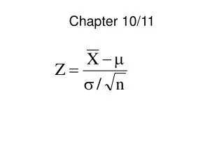

Chapter 10/11
E N D
Presentation Transcript
Chapter 11 • Type 1 error: reject null hypothesis – send a innocent man to jail
Type 2 error: don’t reject a false null hypothesis. Guilty man goes free. Our original hypothesis… our new assumption…
Chapter 11 • The p-value of a test is the probability of observing a test statistic at least as extreme as the one computed given that the null hypothesis is true. p-value P-value =.0069 Z=2.46
Chapter 11 – Type II Error • Recall Example 11.1… • H0: µ = 170 • H1: µ > 170 • At a significance level of 5% we rejected H0 in favor of H1 since our sample mean (178) was greater than the critical value of (175.34). In the question – they will have to give you the new mean to test. ($180 mean) • β= P( x < 175.34, given that µ = 180), thus…
Example 11.1 (revisited) Our original hypothesis… our new assumption… Chance we send a guilty man free
Chapter 12: Inference about a pop Student-t distribution: 1. for a population (defined as greater then 20 times the sample population!) 2. Interval data 3. Used when you have no standard dev
Chapter 12: Inference about a pop • T-test Mean: used to get information about a sample of results comparing it to some mean value that you need to provide (u = 450 boxes an hour). • It will give you ‘t’ stat – to see if it is greater then critical t value (eg 1.656 – defined by confidence level and degrees of freedom. 1.89 > 1.67
Chapter 12: Inference about a pop • Student t-distribution is ROBUST – if nonnormal, results of t-test and con interval estimate are still valid unless it is ‘extremely nonnormal’.
Chapter 12: Inference about a pop Estimator of u (using t-estimate w added finite pop) Estimating Totals for Finite Populations: take the t-estimate and multiply the limits by the population size to get the limits of the mean for the population. (t-estimate value of all purchases in store) Estimate of the total amount:
Chapter 12: Inference about a pop • Inference: Population Proportion (z-test: proportion) • Counting number of occurrences of each value (voting poll, to see probability of x winning, using the sample proportion of votes). • NOMINAL data (voting, fruit, colours) • Describing a Population • sampling distribution is approx normal with mean of ‘p’ if n*p and n(1-p) BOTH > 5.
Chapter 12: Inference about a pop In Question screen, test was looking for conservative votes Q1. Did their total vote tally differ? Did they? P-value: Q2. Did Conservatives get more then Liberals? Did he? P-value: Q2. Did the Liberals get more then the Conservatives? Did he? P-value: NO .0764 YES .0382 NO .9618
Chapter 12: Inference about a pop Population Estimator (estimator of p) • just like t-estimate, by getting the LCL and UCL, you can multiply by the population to see how many watched or visited a certain tv show (this instance how many watched friends at 8pm) Multiply 100,000 viewers By .0991 and ,1269 to get Lower and upper limit
Chapter 13(inference about comparing two population) 2 populations, can get difference between 1) means 2) ratio of 2 variances 3) proportions
Chapter 13 (inference about comparing two population) 1. Difference between Means (t-test: two samples assuming unequal/equal variances) • These are independent samples mutually exclusive samples (if they were related, you would use a matched pair technique!) • use t-test • SO 2 cases: • Equal variances • Unequal variances • TO FIND OUT IF EQUAL/UNEQUAL: • Will tell you in question • Look at F-Estimator of ratio of 2 variances • Look on the equal/unequal chart given to see if their variances are greater then a 2:1 ratio – if so = UNEQUAL variaces! • Look to compare the t-stat and the t critical value (for 1 or 2 tail test) on chart. If outside value, then reject null.
Chapter 13 (inference about comparing two population) t-test: Equal/unequal variances t-test of Q. Calories eaten at lunch by 2 separate populations – do they differ?
Chapter 13 (inference about comparing two population) • t-estimator – 2 means (unequal/equal variances) • - same as before, just with upper/lower levels of means * population. NOTE: If populations are very nonnormal and equal variances, then you can use Wilxocon rank sum test. If, unequal variance – there is no test!
Chapter 13 (inference about comparing two population) Equal Variances Chart (times to assemble)
Chapter 13 (inference about comparing two population) Matched Pairs Experiment (t-test and estimator of UD ) • if you can find a way to pair the independent samples, then you can use this method. Just cause they have the same number of samples, doesn’t mean they are matched, even if they are ordered, they NEED to be matched on another variable (gpa buckets etc).
Chapter 13 (inference about comparing two population) Matched Pairs Experiment (t-test and estimator of UD ) Q. Do finance majors make more then marketing? Take 25 random people – then do t-test of equal/unequal variances. BUT, in this they took 25 buckets of GPA’s and took 1 random person from each range of GPA = matched pairs.
Chapter 13 (inference about comparing two population) 2) Inference about the ratio of two variances: (F-test: two sample for variances) • This is to see if the variances of 2 variances are different. The null is always σ2/ σ2 = 1. • If you want to show if different then want two tail ‘does not equal’ test. • PRINTOUT will give you one tail p-value (will need to double to get p-value)
Chapter 13 (inference about comparing two population) • F-Estimator of ratio of 2 variances – same as usual That is, we estimate that σ12 / σ22 lies between .2374 and .6594 Note that one (1.00) is not within this interval…
Chapter 13 (inference about comparing two population) • 3) Inference about the difference between population proportions (with nominal data) – z-test of p1 – p2 • Using nominal data, so win/lose categories – to give you proportions. • same restriction of the p*n and p*(1-n) > 5 (but now for both populations) • depending on null hypothesis, there are 2 different formula (one for =0 and one for = D (not 0) – look to the hypothesized mean line in table.
Chapter 13 (inference about comparing two population) Z-test of p1 – p2 type 1 - eg: testing for the proportion of a certain product being sold in 2 different stores – with a difference of 0 (so seeing if supermarket 1 sold more then supermarket 2)
Chapter 13 (inference about comparing two population) Z-test of p1 – p2 type 2 - eg: testing for the proportion of a certain product being sold in 2 different stores – with a difference of 3% (so seeing if supermarket 1 sold 3% more then supermarket 2)
Chapter 15 : Analysis of Variance • comparing 2 or more population of INTERVAL data • determine whether differences exist between population means • done by analyzing sample variance. • ANOVA uses the errors within groups and between groups, to essentially determine if the means differ. 3 TYPES OF ANOVA: • Single Factor: For populations which have only 1 factor that you are comparing them against, then you use the ANOVA: Single Factor. This is like comparing sales from 3 cities with the factor being the marketing strategy. • TwoFactor: When you have 2 or more independent samples with 2 factors (comparing 3 cities based on marketing strategy and marketing medium) – NOT ON EXAM • Randomized Block (two-way Anova): when you have 1 factor, but the samples in each treatment are groups according to some variable (like age/weight, or gpa).
Chapter 15 : Analysis of Variance 1. SINGLE FACTOR • Condition: • MST/MSE = F compare this value with F crit on the chart. If F value is greater then F-crit then the means differ. • REQUIRED CONDITIONS: the random variables must be normally distributed with equal variances. Check by histograms. If NOT normal, then you can Kruskal-Wallis Test. • If pop variances are unequal – we have NO test!!
Chapter 15 : Analysis of Variance Single Factor: • Comparing 3 independent populations, with the factor being marketing strategy. Q. Is there enough evidence to support that the sales of this product differ? All this says is that at least 2 of the means differ!
Chapter 15 : Analysis of Variance Must be normal and equal variances: • If nonnormal, replace test with Kruskal-Wallis test (making the numbers ordinal). • If unequal variances – we CANNOT DO! All this says is that at least 2 of the means differ!
Chapter 15 : Analysis of Variance RANDOMIZED BLOCK (Two-Factor Without Replication) • Here you are only comparing across 1 factor essentially, but splitting the samples into blocks. • SO: • MST/MSE = F still holds if wanting to compare treatments (standard case). But if you want to compare between the BLOCKS – then: • F = MST/MSB (ROW ERROR). • In the chart, you will get the variation of between the rows (between the buckets, which we usually aren’t looking for, cause we know they will be different – but still testable (ROWS Error)), and variation between columns (what we are looking for – difference between treatments (COLUMN Error)). Compare the F value and the F-crit. • Requirement: Must be normal, and equal var. If nonnormal – use Friedman Test
Chapter 15 : Analysis of Variance Q: testing 4 drugs, with 25 men – who are paired with someone else in same age/weight category. Their cholesterol different was measured (interval). Are any drugs more successful then others? Q2. Does the success of the drug differ between age/weight?
Summary of ANOVA two-factor analysis of variance one-way analysis of variance two-way analysis of variance a.k.a. randomized blocks
Ch 15 : Multiple Comparisons When we conclude from the one-way analysis of variance that at least two treatment means differ (i.e. we reject the null hypothesis that H0) we often need to know which treatment means are responsible for these differences. We will examine three statistical inference procedures that allow us to determine which population means differ: • Fisher’s least significant difference (LSD) method • Bonferroni adjustment, and • Tukey’s multiple comparison method.
Ch 15 : Multiple Comparisons Fisher’s Least Significant Difference (LSD) • Compare the mean difference of all combinations with the calculated LSD • Take the ABSOLUTE value to see if bigger.
Ch 15 : Multiple Comparisons • Bonferri Adjustment • It takes the LSD format, but instead of using the sig level as is, it divides it by k(k-1)/2 – k being treatments, to get a smaller sig level – and lower change of type 1 error. • Use the Multiple Comparisons method, but you need to PRE-adjust the sig level before entering it in – it is still a LSD method,
Ch 15 : Multiple Comparisons • Tukey’s Multiple Comparison Method (w) • Same concept, see which is higher RULE OF THUMB: if you have 2/3 pairwise comparisons use Bonferroni’s comparison. If you want to compare ALL possible combinations, use tukey’s.
Chapter 16: Chi-Squared Tests • Goodness of Fit Test – used in 2 ways: • used to describe one population of data with more then 2 nominal options (no heads/tails, but rock/paper/scissor) • trials must be independent • must have expected frequency > 5 for each (n*p) • have a null hypoth being equal to the p*n for each option, and goodness of fit test determines of the actual results differ from them. • used to determine if two classifications of a pop are statistically independent- also interpreted as a comparison of 2+ populations Given frequencies of .45, .40, and .15, - expected frequency. This test compares the expected to the actual, and gives p-value.
Chapter 16: Chi-Squared Tests • Chi-Squared test of a Contingency Table • is there enough evidence to infer that two nominal variables are related or • to infer that differences exist between two or more populations of nominal data.
Chapter 17: Linear Regression and Correlation • Regression: USED TO: analysis the relationship between interval variables. Deterministic Model: set of equations to mathematically determine the value of the dependent variable from the values of the independent. Probabilistic Model: method used to capture the randomness (try to fit an equation relating size of houses and cost of houses) Deterministic Model: y = 200 + 4x – we know that price of a car goes up by $4 for each horse power unit. Probabilistic Model y = 200 + 4x + ε (error) – this represents the real world variability.
Chapter 17: Linear Regression and Correlation • Eg: resell value of car with x miles on the odometer Standard Error (Se) = how good the error in the points is (relate this to the mean) Coefficient of Determination (R^2) = how much of the variation is due to the independent variable (if 1 – no error, and all variation due to indep, if 0 – no linear relationship between variables, and all error).
Chapter 17: Linear Regression and Correlation • Coorelation (Pearson) • to see the direction of the relationship, coorelation will be between -1 and 1 • do a 2 tail test if you want to know if there is a relationship • do a 1 tail test if you want to know if there is a positive/negative relationship
Chapter 17: Linear Regression and Correlation Prediction Interval Method • To find out the expected value of an individual item (prediction interval) or the expected value of the mean of a population (confidence interval estimate) • The confidence interval estimate of the expected value of y will be narrower than the prediction interval for the same given value of x and confidence level. This is because there is less error in estimating a mean value as opposed to predicting an individual value. Point Prediction Estimate of the range of 1 population Prediction Interval The interval that the mean of a large number of trails will fall in. Confidence Interval Estimator of the mean price
Chapter 18: Multiple Regression (multiple variables, all first-order) Eg: Hotel profit margin – based on 6 factors.
Chapter 19: Model Building • Checking the regression tool’s output… The model fits the data well and its valid… Uh oh. multicollinearity
Chapter 21: Nonparametic Techniques • USED TO: • Testing characteristics of ORDINAL DATA • Used for when interval data is NONNORMAL – so all about seeing where the population values are when comparing 2 populations
Chapter 21: Nonparametic Techniques Wilcoxon Rank Sum Test • compare 2 pop’s • ordinal (or nonnormal interval) • independent samples You rank all the values from both populations, and rank them from lowest to highest and sum up each population by the ranks of each pop’s values. You need to compare the z-stat and the z-critical for one-tail / two-tail – depending if you want to see if the populations locations are different (two-tail) or if one is greater then the other (one-tail). NOTE: need to have identical spreads (variance) and shape (distribution)
Chapter 21: Nonparametic Techniques Eg: testing quality of new painkiller vs plain old aspirin. It ranks the answers, and sums the ranks and the test determines if there is a difference. This is testing to see if the new one IS better the one one – 1 tail test. p-value compare…
Chapter 21: Nonparametic Techniques Sign Test • compare 2 pop’s • ordinal or interval (nonnormal) • samples are MATCHED PAIRS • must be similar in shape and spread • Of each match, denote a -1 or 1 (which one is bigger). • Look to the z-stat /p-value to see if bigger then z-crit (one or two tail)
Chapter 21: Nonparametic Techniques Eg: testing to see if european cars are more comfortable then american cars. p-value compare…
Chapter 21: Nonparametic Techniques • Wilcoxon Signed Rank Sum Test • used only for comparing • 2 populations • nonnormal interval data • matched pairs • Compute paired differences • Rank absolute values of differences’sum the ranks of +ive and –ve differences • Use Rank Sum Test and compare z-stat / p-value.