Introduction to Bioinformatics
520 likes | 587 Vues
Learn about data clustering and classification methods in bioinformatics to find patterns in biological data, understand relationships, and classify data using different algorithms like hierarchical clustering, k-means, and nearest neighbors. Explore various distance metrics and similarity matrices for grouping similar genes and proteins. Understand the fundamentals of supervised and unsupervised classification in bioinformatics.

Introduction to Bioinformatics
E N D
Presentation Transcript
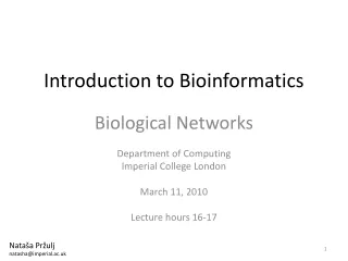
Introduction to Bioinformatics Biological Networks Department of Computing Imperial College London March 11, 2010 Lecture hours 16-17 Nataša Pržulj natasha@imperial.ac.uk
Data Clustering • find relationships and patterns in the data • get insights in underlying biology • find groups of similar genes/proteins/samples • deal with numerical values of biological data • they have many features (not just colour)
Data Clustering • There are many possible distance metrics between objects • Theoretical properties of distance metrics, d: • d(a,b) >= 0 • d(a,a) = 0 • d(a,b) = 0 a=b • d(a,b) = d(b,a) – symmetry • d(a,c) <= d(a,b) + d(b,c) – triangle inequality
Clustering Algorithms Example distances: • Euclidean (L2) distance • Manhattan (L1) distance • Lm: (|x1-x2|m+|y1-y2|m)1/m • L∞: max(|x1-x2|,|y1-y2|) • Inner product: x1x2+y1y2 • Correlation coefficient • For simplicity we will concentrate on Euclidean and Manhattan distances
Clustering Algorithms Distance/Similarity matrices: • Clustering is based on distances – distance/similarity matrix: • Represents the distance between objects • Only need half the matrix, since it is symmetric
Clustering Algorithms Hierarchical Clustering: • Scan dist. matrix for the minimum • Join items into one node • Update matrix and repeat from step 1
Clustering Algorithms Hierarchical Clustering: • Distance between two points – easy to compute • Distance between two clusters – harder to compute: • Single-Link Method / Nearest Neighbor • Complete-Link / Furthest Neighbor • Average of all cross-cluster pairs
Clustering Algorithms Hierarchical Clustering: • 1. Example: Single-Link (Minimum) Method: Resulting Tree, or Dendrogram:
Clustering Algorithms Hierarchical Clustering: • 2. Example: Complete-Link (Maximum) Method: Resulting Tree, or Dendrogram:
Clustering Algorithms Hierarchical Clustering: In a dendrogram, the length of each tree branch represents the distance between clusters it joins. Different dendrograms may arise when different Linkage methods are used.
Clustering Algorithms K-Means Clustering: • Basic Ideas : use cluster centroids (means) to represent cluster. • Assigning data elements to the closet cluster (centroid). • Goal: Minimize intra-cluster dissimilarity.
Clustering Algorithms K-Means Clustering Example:
Clustering Algorithms • Differences between the two clustering algorithms: • Hierarchical Clustering: • Need to select Linkage Method • to perform any analysis, it is necessary to partition the dendrogram into k disjoint clusters, cutting the dendrogram at some point. A limitation is that it is not clear how to choose this k • K-means: Need to select K • In both cases: Need to select distance/similarity measure
Clustering Algorithms Nearest neighbours clustering:
Clustering Algorithms Nearest neighbours clustering: Example: Pros and cons: No need to know the number of clusters to discover beforehand (different than in k-means and hierarchical). 2. We need to define the threshold .
Clustering Algorithms k-nearest neighbors clustering -- classification algorithm, but we use the idea here to do clustering: • For point v, create the cluster containing v and top k closest points to v (closest training examples); e.g., based on Euclidean distance. • Do this for all points v. • All of the clusters are of size k, but they can overlap. • The challenge: choosing k.
What is Classification? The goal of data classification is to organize and categorize data in distinct classes. • A model is first created based on the data distribution. • The model is then used to classify new data. • Given the model, a class can be predicted for new data. Example: Application: medical diagnosis, treatment effectiveness analysis, protein function prediction, interaction prediction, etc.
What is Clustering? • There is no training data (objects are not labeled) • We need a notion of similarity or distance (over what features?) • Should we know a priori how many clusters exist? • How do we characterize members of groups? • How do we label groups?
Supervised and Unsupervised Supervised Classification = Classification • We know the class labels and the number of classes Unsupervised Classification = Clustering • We do not know the class labels and may not know the number of classes
Classification vs. Clustering (we can compute it without the need of knowing the correct solution)
Classification is a 3-step process • Model Construction (Learning): • Each tuple is assumed to belong to a predefined class, as determined by one of the attributes, called the class label. • The set of all tuples used for construction of the model is called the training set. • The model is presented in forms such as: • Classification rules (IF-THEN statements) • Mathematical formulae
Classification is a 3-step process • Model Evaluation (Accuracy): • Estimate accuracy rate of the model based on a test set. • The known label of test sample is compared with • the classified result from the model. • Accuracy rate is the percentage of test set samples • that are correctly classified by the model. • Test set is independent of training set, otherwise • over-fitting will occur.
Classification is a 3-step process • Model Use (Classification): The model is used to classify unseen objects. • Give a class label to a new tuple • Predict the value of an actual attribute
k-Nearest Neighbours (k-NN) Classification • In k-nearest-neighbour classification, the training dataset is used to classify each member of a "target" dataset. • There is no model created during a learning phase but the training set itself. • It is called a lazy-learningmethod. • Rather than building a model and referring to it during the classification, k-NN directly refers to the training set for classification.
Simple Nearest Neighbour Classification • It is very simple. The training is nothing more than sorting the training data and storing it in a list. • To classify a new entry, this entry is compared to the list to find the closest record, with value as similar as possible to the entry to classify (i.e., nearest neighbour). The class of this record is simply assigned to the new entry. • Different measures of similarity or distance can be used.
k-Nearest Neighbours (k-NN) Classification • The k-Nearest Neighbour is a variation of Nearest Neighbour. Instead of looking for only the closest record to the entry to classify, we look for the k records closest to it. • To assign a class label to the new entry, from all the labels of the k nearest records we take the majority class label. • Nearest Neighbour is a case of k-Nearest Neighbours with k=1.
Correctness of methods • Clustering is used for making predictions: • E.g., protein function, involvement in disease, interaction prediction. • Other methods are used for classifying the data (have disease or not) and making predictions. • Have to evaluate the correctness of the predictions made by the approach. • Commonly used method for this is ROC Curves.
Correctness of methods Definitions (e.g., for PPIs): • A true positive (TP) interaction: • an interaction exists in the cell and is discovered by an experiment (biological or computational). • A true negative (TN) interaction: • an interaction does not exist and is not discovered by an experiment. • A false positive (FP) interaction: • an interaction does not exist in the cell, but is discovered by an experiment. • A false negative (FN) interaction: • an interaction exists in the cell, but is not discovered by an experiment.
Correctness of methods • If TP stands for true positives, FP for false positives, TN for true negatives, and FN for false negatives, then: • Sensitivity = TP / (TP + FN) • Specificity = TN / (TN + FP) • In other words, sensitivity measures the fraction of items out of all possible ones that truly exist in the biological system that our method successfully identifies (fraction of correctly classified existing items), while • specificity measures the fraction of the items out of all items that truly do not exist in the biological system for which our method correctly determines that they do not exist (fraction of correctly classified non-existing items). • Thus, 1-specificity measures the fraction of all non-existing items in the system that are incorrectly identified as existing.
ROC Curve • Receiver Operating Curves (ROC curves) provide a standard measure of the ability of a test to correctly classify objects. • E.g., the biomedical field uses ROC curves extensively to assess the efficacy of diagnostic tests in discriminating between healthy and diseased individuals. • ROC curve is a graphical plot of the true positive rate, i.e., sensitivity, vs. false positive rate, i.e., (1−specificity), for a binary classifier system as its discrimination threshold is varied (see above for definitions). • It shows the tradeoff between sensitivity and specificity (any increase in sensitivity will be accompanied by a decrease in specificity). • The closer the curve follows the left-hand border and then the top border of the ROC space, the more accurate the test; the closer the curve comes to the 45-degree diagonal of the ROC space, the less accurate the test. The area under the curve (AUC) is a measure of a test’s accuracy.
ROC curve Example: • Embed nodes of a PPI network into 3-D Euclidean unit box (use MDS – not required in this class, see reference in the footer if interested) • Like in GEO, choose a radius r to determine node connectivity • Vary r between 0 and sqrt(3) (diagonal of the box) • r=0 makes a graph with no edges (TP=0, FP=0) • r=sqrt(3) makes a complete graph (all possible edges, FN=TN=0) • For each r in [0, sqrt(3)]: • measure TP, TN, FP, FN • compute sensitivity and 1- specificity • draw the point • Set of these points is the ROC curve Note: • For r=0, sensitivity=0 and 1-specificity=0, since TP=0, FP=0 (no edges) • For r=sqrt(3), sensitivity=1 and 1-specificity=1 (or 100%), since FN=0, TN=0 Sensitivity = TP / (TP + FN) Specificity = TN / (TN + FP) D. J. Higham, M. Rasajski, N. Przulj, “Fitting a Geometric Graph to a Protein-Protein Interaction Network”, Bioinformatics, 24(8), 1093-1099, 2008.
Types of Biological Network Comparisons: • Molecular networks: the backbone of molecular activity within the cell • Comparative approaches toward interpreting them -- contrasting networks of • different species • molecular types • under varying conditions • Comparative biological network analysis and its applications to elucidate cellular machinery and predict protein function and interactions. Sharan and Ideker (2006) Nature Biotechnology24(4): 427-433
Types of Biological Network Comparisons: • Data on molecular interactions are increasing exponentially • This flood of information parallels that seen for genome sequencing in the recent past • Presents exciting new opportunities for understanding cellular biology and disease in the future • The challenge: develop new strategies and theoretical frameworks to filter, interpret and organize interaction data into models of cellular function
Types of Biological Network Comparisons: • As with sequences, comparative/evolutionary view is a powerful base to address this challenge • We will survey computational methodology it requires and biological questions it may be able to answer • Conceptually, network comparison is the process of contrasting two or more interaction networks, representing different: • species, • conditions, • interaction types, or • time points
Types of Biological Network Comparisons: • Based on the found similarities, answer a number of fundamental biological questions: • Which proteins, protein interactions and groups of interactions are likely to have equivalent functions across species? • Can we predict new functional information about proteins and interactions that are poorly characterized? • What do these relationships tell us about the evolution of proteins, networks, and whole species? 39
Types of Biological Network Comparisons: • Noise in the data – screens for PPI detection report large numbers of false-positives and negatives: • Which interactions represent true binding events? • Confidence measures on interactions should be taken into account before network comparison. • However, since a false-positive interaction is unlikely to be reproduced across the interaction maps of multiple species, network comparison itself increases confidence in the set of molecular interactions found to be conserved 40 40
Types of Biological Network Comparisons: • Such questions have motivated 3 types (modes) of comparative methods: • Network alignment • Network integration • Network querying 41 41 41 41
Types of Biological Network Comparisons: • Network alignment: • The process of overall comparison of two or more networks to identify regions of similarity and dissimilarity • Commonly applied to detect subnetworks that are conserved across species and hence likely to present true functional modules 42 42 42 42 42
Types of Biological Network Comparisons: • Network integration: • The process of combining several networks encompassing interactions of different types over the same set of elements (e.g., PPI and genetic interactions) • To study their interrelations • Can assist in predicting protein interactions and uncovering protein modules supported by interactions of different types • The main conceptual difference from network alignment: • the integrated networks are defined on the same set of elements. 43 43 43 43 43 43
Types of Biological Network Comparisons: • Network querying: • A given network is searched for subnetworks that are similar to a subnetwork query of interest • This basic database search operation is aimed at transferring biological knowledge within and across species • Summary: 44 44 44 44 44 44 44
1. Network Alignment • Finding structural similarities between two networks 45 45 45
A B 1 2 C D 3 4 G H 1. Network Alignment • Recall • Subgraph isomorphism (NP-complete): • An isomorphism is a bijection between nodes of two networks G and H that preserves edge adjacency • Exact comparisons inappropriate in biology (biological variation) • Network alignment • More general problem of finding the best way to “fit” G into H even if G does not exist as an exact subgraph of H A 1 B 2 C 4 D 3 46 46 46 46
1. Network Alignment • Methods vary in these aspects: • Global vs. local • Pairwise vs. multiple • Functional vs. topological information 48 48 48 48 48 48
1. Network Alignment • Methods vary in these aspects: • Global vs. local • Pairwise vs. multiple • Functional vs. topological information • Local alignment: • Mappings are chosen independently for each region of similarity • Can be ambiguous, with one node having pairings in different local alignments • Example algorithms: • PathBLAST, NetworkBLAST, MaWISh, Graemlin 49 49 49 49 49
1. Network Alignment • Methods vary in these aspects: • Global vs. local • Pairwise vs. multiple • Functional vs. topological information • Global alignment: • Provides a unique alignment from every node in the smaller network to exactly one node in the larger network • May lead to inoptimalmachings in some local regions • Example algorithms: • GRAAL, IsoRank, IsoRankN, Extended Graemlin 50 50 50 50 50 50