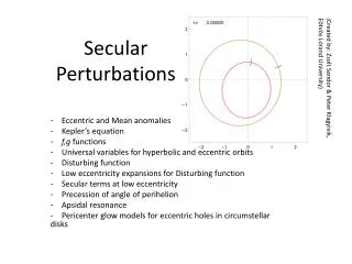
Secular Perturbations

(Created by: ZsoltSandor & Peter Klagyivik, EötvösLorand University) Secular Perturbations Eccentric and Mean anomalies Kepler’s equation f,g functions Universal variables for hyperbolic and eccentric orbits Disturbing function Low eccentricity expansions for Disturbing function Secular terms at low eccentricity Precession of angle of perihelion Apsidal resonance Pericenter glow models for eccentric holes in circumstellar disks

Ellipse f = true anomaly Sun is focal point b=semi-minor axis a=semi-major axis b r center of ellipse f a

Ellipse E = Eccentric anomaly f = true anomaly Orbit from center of ellipse a b r f E ae

Relationship between Eccentric, True and Mean anomalies • Using expressions for x,yin terms of true and Eccentric anomalies we find that So if you know E you know f and can find position in orbit Write dr/dtin terms of n, r, a, e Then replace dr/dtwithfunction depending on E, dE/dt

Mean Anomaly and Kepler’s equation • New angle M defined such that or • Integrate dE/dtfinding Kepler’s equation Must be solved to integrate orbit in time. The mean anomaly is not an angle defined on the orbital plane It is an angle that advances steadily in time It is related to the azimuthal angle in the orbital plane, for a circular orbit, the two are the same and f=M

Procedure for integrating orbit or for converting orbital elements to a Cartesian position: • Change t, increase M. • Compute E numerically using Kepler’s equation • Compute f using relation between E and f • Rotate to take into account argument of perihelion • Calculate x,yin plane of orbit • Rotate two more times for inclination and longitude of ascending node to final Cartesian position Kepler’s equation Must be solved to integrate orbit in time.

Inclination and longitude of ascending node • Sign of terms depends on sign of hz. • I inclination. • retrograde orbits have π/2<I<π • prograde have 0<I<π/2 • Ωlongitude of ascending node, where orbit crosses ecliptic • Argument of pericenterωis with respect to the line of nodes (where orbit crosses ecliptic) h angular momentum vector

Orbit in space • line of nodes: intersection of orbital plane and reference plane (ecliptic) • Longitude of ascending node Ω: angle between line of nodes (ascending side) and reference line (vernal equinox) • ω “argument of pericenter” is not exactly the same thing as we discussed before ϖ – longitude of pericenter. ω is not measured in the ecliptic. ϖ=Ω+ω but these angles not in a plane unless I=0 Anomaly : in orbital plane and w.r.t. pericenter Longitude: in ecliptic w.r.t. vernal equinox Argument: some other angle

Orbit in space Rotations • In plane of orbit by argument of pericenterω in (x,y) plane • In (y,z) plane by inclination I • In (x,y) plane by longitude of ascending node Ω • 3 rotations required to compute Cartesian coordinates given orbital elements

Cartesian to orbital elements • To convert from Cartesian coordinates to Orbital elements: • Compute a,eusing energy and angular momentum • Compute inclination and longitude of ascending node from components of angular momentum vector • From current radius and velocity compute f • Calculate E from f • Calculate M from numerical solution of Kepler’s equation • Calculate longitude of perihelion from angle of line of nodes in plane of orbit

The angular momentum vector relation between inclination, longitude of ascending node and angular momentum. Convention is to flip signs of hx,hy if hz is negative Force • component perpendicular to orbital plane • component in orbital plane perpendicular to r • component along radius orthogonal coordinate system

Torque Fr contributes no torque To vary |h| a torque in z direction is need, only depends on Fθ - only forces in the plane vary eccentricity To vary direction of h a force in direction of z is needed instantaneous variations Often integrated over orbit to estimate precession rate

f and g functions • Position and velocity at a later time can be written in terms of position and velocity at an earlier time. Numerically more efficient as full orbital solution not required.

Differential form of Kepler’s equationProcedure for computing f,g functions • Compute a, e from energy and angular momentum. • Compute E0 from position • Compute ΔE by solving numerically the differential form of Kepler’s equation. • Compute f,g, find new r. • Compute • One of these could be computed from the other 3 using conservation of angular momentum Subtract Kepler’s equation at two different times to find: )

Universal variables • Desirable to have integration routines that don’t require testing to see if orbit is bound. • Converting from elliptic to hyperbolic orbits is often of matter of substituting sin, cos for sinh, cosh • Described by Prussing and Conway in their book “Orbital Mechanics”, referring to a formulation due to Battin. x is determined by Solving a differential form of Kepler’s equation in universal variables

Analogy

Differential Kepler’s equation in universal variables • x solves (universal variable differential Kepler equation • Special functions needed:

Solving Kepler’s equation • Iterative solutions until convergence • Rapid convergence (Laguerre method is cubic) • Only 7 or so iterations needed for double precision (though this could be tested more rigorously and I have not written my routines with necessarily good starting values).

Orbital elements • a,e,IM,ω,Ω (associated angles) • As we will see later on action variables related to the first three will be associated with action angles associated with the second 3. • For the purely Keplerian system all orbital elements are constants of motion except M which increases with • Problem: If M is an action angle, what is the associated momentum and Hamiltonian?

Keplerian Hamiltonian • Problem: If M is an action angle, what is the associated action momentum and Hamiltonian? • Assume that • From Hamilton’s equations • Energy

Keplerian Hamiltonian • Solving for constants • Unperturbed with only 1 central mass • We have not done canonical transformations to do this so not obvious we will arrive exactly with these conjugate variables when we do so.

Hamiltonian formulation • Poincare coordinates

Working in Heliocentric coordinates • Consider a central stellar mass M*, a planet mp and a third low mass body. “Restricted 3 body problem” if all in the same plane • We start in inertial frame (R*, Rp, R) and then transform to heliocentric coordinates (rp, r) Replace accelerations in inertial frame with expressions involving acceleration of star. Then replace acceleration of star with this so we gain a term

Disturbing function New potential, known as a disturbing function – due to planet Gradient w.r.t to r not rp Force from Sun • Indirect term -- because planet has perturbed position of Sun and we are not working an inertial frame but a heliocentric one— • - Reduces 2:1 resonance strength. • - Contributes to slow m=1 eccentric modes of self-gravitating disks Direct term

Direct and Indirect terms • For a body exterior to a planet it is customary to write • For a body interior to a planet: • In both cases the direct term • Convention ratio of semi-major axes

Lagrange’s Planetary equations • One can use Hamilton’s equations to find the equations of motion • If written in terms of orbital elements these are called Lagrange’s equations • These are time derivatives of the orbital elements in terms of derivatives of the disturbing function • To relate Hamilton’s equations to Lagrange’s equations you can use the Jacobian of derivatives of orbital elements in terms of Poincare coordinates

Lagrange’s equations where ε is mean longitude at t=0 or at epoch

Secular terms • Expansion to second order in eccentricity • Neglecting all terms that contain mean longitudes • Should be equivalent to averaging over mean anomaly • Indirect terms all involve a mean longitude so average to zero Laplace coefficients which are a function of α I have dropped terms with inclination here – there are similar ones with inclination Similar term for other body

Evolution in e • Lagrange’s equations (ignoring inclination) • Convenient to make a variable change • Writing out the derivatives

Equations of motion • For two bodies • With solutions depending on eigenvectors es,ef and eigenvaluesgs,gfof matrix A (s,f: slow and fast) • Slow: both components of eigenvector with same sign, • Fast: components of eigenvector have opposite sign

Solutions One eigenvector Both eigenvectors ef es es

Both objects apsidal alignment es,1 ef,1 es,2 ef,2 Anti aligned, fast, Δϖ=π Aligned and slow, Δϖ=0 How can angular momentum be conserved with this?

Predicting evolution from orbital elements • Unknowns • magnitudes of the 2 eigenvectors • 2 phases • From current orbital elements

Animation of the eccentricity evolution of HD 128311(Created by: ZsoltSandor & Peter Klagyivik, EötvösLorand University)

Both together in a differential coordinate system radius = e1e2 Apsidal aligned, non circulating, can have one object with nearly zero eccentricity. “Libration” fast only Slow only Circulating Note orbits on this plot should not be ellipses

Examples of near separatrix motionFor exatrasolar planets Libration Circulation Δϖ Δϖ different lines consistent with data e e one planet Time  Time  In both cases one planet drops to near zero eccentricity

From Barnes and Greenberg 08 Δϖ e

Simple Hamiltonian systemsTerminology Harmonic oscillator I  p q Stable fixed point Libration Oscillation Pendulum p Separatrix

Multiple planet systemsRV systems • No obvious correlation mass ordering vs semi-major axis • Mostly 2 planets but some with 3, 5 • Eccentric orbits, but lower eccentricity than single planet systems • Rasio, Ford, Barnes, Greenberg, Juric have argued that planet scattering explains orbital configurations • Subsequent evolution of inner most object by tidal forces • Many systems near instability line • Lower eccentricity for multiple planet systems • Lower mass systems have lower eccentricities

Mass and Eccentricity distribution of multiple planet systems High eccentricity planets tend to reside in single planetary systems

Hamiltonian view Poincaré momentum massless object near a single planet μ = mp/M* - Aligned with planet Eccentricity does not depend on planet mass but does on planet eccentricity Fixed point at

Expand around fixed point • First transfer to canonical coordinates using h,k • Then transfer to coordinate system with a shift h’=h-hf, k’=k-kf • Harmonic motion about fixed point: that’s the free eccentricity motion

efree eforced Free and Forced eccentricity • Massless body in proximity to a planet Force eccentricity depends on planet’s eccentricity and distance to planet but not on planet’s mass. Mass of planet does affect precession rate. Free eccentricity size can be chosen.

Secular problem with free and forced eccentricities

Pericenter Glow • Mark Wyatt, developed for HR4796A system, later also applied to Fomalhaut system

Multiple Planet systemHamiltonian view • Single interaction term involving two planets • All semi-major axes and eccentricities are converted to mometa • Three low order secular terms, involving Γ1,Γ2,(Γ1Γ2)1/2 • Hamilton’s equation give evolution consistent with two eigenvectors previously found.

Epicyclic approximation These cancel to be consistent with a circular orbit

Epicyclic frequency to higher order in epicyclic amplitude (Contopoulos)

More generally on epicyclic motion Low epicyclic amplitude expansion As long as there are no commensurabilities between radial oscillation periods and orbital period this expansion can be carried out For a good high epicyclic amplitude approximation see a nice paper by Walter Dehnen using a second order expansion but of the Hamiltonian times a carefully chosen radial function

Low eccentricity Expansions • Functions of radius and angle can be written in terms of the Eccentric anomaly is an odd function This can be shown by integrating and using Kepler’s equation (see page 38 M+D) Bessel function of the first kind

Secular Perturbations