Download
1 / 20
200 likes | 322 Vues
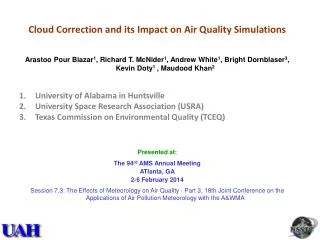
Cloud Correction and its Impact on Air Quality Simulations Arastoo Pour Biazar 1 , Richard T. McNider 1 , Andrew White 1 , Bright Dornblaser 3 , Kevin Doty 1 , Maudood Khan 2 University of Alabama in Huntsville University Space Research Association (USRA)

E N D
Cloud Correction and its Impact on Air Quality Simulations • Arastoo Pour Biazar1, Richard T. McNider1, Andrew White1, Bright Dornblaser3, Kevin Doty1 , Maudood Khan2 • University of Alabama in Huntsville • University Space Research Association (USRA) • Texas Commission on Environmental Quality (TCEQ) • Presented at: • The 94rd AMS Annual Meeting • ATlanta, GA • 2-6 February 2014 • Session 7.3: The Effects of Meteorology on Air Quality - Part 3, 18th Joint Conference on the Applications of Air Pollution Meteorology with the A&WMA
Background & Motivation: • Clouds greatly impact tropospheric chemistry by altering dynamics as well as atmospheric chemical processes: • Altering photochemical reaction rates and thereby impacting oxidant production. • Impacting surface insolation and temperature and thereby altering the emissions of key ozone precursors (namely biogenic hydrocarbons and nitrogen oxide.) • Impacting boundary-layer development, vertical mixing, and causing deep vertical mixing of pollutants and precursors. • Impacting the evolution and recycling of aerosols. • Impacting aqueous phase chemistry and wet removal. • Causing lightning and generating nitrogen. • Unfortunately, numerical meteorological models still have difficulty in creating clouds in the right place and time compared to observed clouds.This is especially the case when synoptic-scale forcing is weak, as often is the case during air pollution episodes.
Background & Motivation … • The errors in simulated clouds is particularly important in State Implementation Plan (SIP) modeling where the best representation of physical atmosphere is required. • Previous attempts at using satellite data to insert cloud water have met with limited success. • Studies have indicated that adjustment of the model dynamics and thermodynamics is necessary to fully support the insertion of cloud liquid water in models (Yucel, 2003). • Jones et al., 2013, assimilated cloud water path in WRF and realized that the maximum error reduction is achieved within the first 30 minutes of forecast. • Assimilation of radar observations (Dowell et al., 2010) miss the non-precipitating clouds. • Assimilation of observed cloud optical depth (Lauwaet et al., 2011) has also shown to improve model performance by improving the model surface temperatures.
ASSIM OBSERVED CNTRL Under-prediction UAH Approach: • Objective: to improve model location and timing of clouds in the Weather Research and Forecast (WRF) model by assimilating GOES observed clouds. • Since for air quality, non-precipitating clouds are just as important as precipitating clouds, our metric for success should indicate the radiative impact of clouds. • Approach: Create an environment in the model that is conducive to clouds formation/removal through adjusting wind and moisture fields and to improve the ability of the WRF modeling system to simulate clouds through the use of observations provided by the Geostationary Operational Environmental Satellite (GOES). Correcting for the radiative impact of clouds corrected 38 ppb under-prediction. (Pour-Biazar et al 2007)
UAH Approach … W > 0 W < 0 Photolysis Adjustment (CMAQ) Dynamical Adjustment Cloud top Determined from satellite IR temperature SUN c h BL OZONE CHEMISTRY O3 + NO -----> NO2 + O2 NO2 + h (<420 nm) -----> O3 + NO VOC + NOx + h-----> O3 + Nitrates (HNO3, PAN, RONO2) Cloud albedo, surface albedo, and insolation are retrieved based on Gautier et al. (1980), Diak and Gautier (1983). From GOES visible channel centered at .65 µm. • Use satellite cloud top temperatures and cloud albedoes to estimate a TARGET VERTICAL VELOCITY (Wmax). • Adjust divergence to comply with Wmax in a way similar to O’Brien (1970). • Nudge model winds toward new horizontal wind field to sustain the vertical motion. g g Surface
Implementation in WRF • Focusing on daytime clouds, analytically estimate the vertical velocity needed to create/clear clouds. • Under-prediction: Lift a parcel to saturation. Over-prediction: Move the parcel down to reduce RH and evaporate droplets. • The horizontal wind components in the model are minimally adjusted (O’Brien 1970) to support the target vertical velocity. • REQUIRED INPUTS FOR 1D-VAR: Target W: target vertical velocity (m/s); Target H: where max vertical velocity is reached; Wadj_bot: bottom layer for adjustment; Wadj_top: top layer for adjustment. Implementation in CMAQ • Cloud albedo and cloud top temperature from GOES is used to calculate cloud transmissivity and cloud thickness • The information is fed into MCIP/CMAQ • CMAQ parameterization is bypassed and photolysis rates are then adjusted based on GOES observations: Interpolate in between.
Model Configuration: Modeling Domain 4 km 12 km 36km domain CMAQ
Agreement Index for Measuring Model Performance Underprediction Overprediction Areas of disagreement between model and satellite observation A contingency table can be constructed to explain agreement/disagreement with observation
WRF Results (36-km): Based on Agreement Index Model performance has improved. The improvements are more pronounced at times that the model errors are larger
WRF Results (36-km) … While RMSE for temperature is reduced, cold bias has increased and dry bias has decreased. This points to an inherent problem other than clouds in the model that is making the control simulation dry and cold.
WRF Results (12-km) … Similar to 36-km simulation, for 12-km domain cloud assimilation improved Agreement Index. Using the lateral boundary condition from 36-km simulation with assimilation also improves the model performance.
WRF Results (12-km) … For 12-km domain, unlike the 36-km, temperature shows a positive bias that for some days is improved by assimilation. RMSE and bias for mixing ratio are improved by using the lateral boundary condition from 36-km with assimilation or directly assimilating GOES observations.
CMAQ Results (36-km): SATCLD SIMULATION CONTROL SIMULATION Transmissivity CNTRL too opaque compared to satellite NO2 photolysis rate Large differences due to cloud errors
Difference in NO2 photolysis rates for selected days(CNTRL-SATCLD) Difference in NO2 photolysis rates between control simulation and the simulation using observed clouds (CNTRL-SATCLD) for August 19, 21,22, and 29, 2006. Clouds in control simulation are more spread out and cover large areas (more opaque compared to observation). Over-prediction of Clouds by CNTRL Under-prediction of Clouds by CNTRL
CNTRL SATCLD Under prediction for higher ozone concentrations is slightly improved due to GOES cloud adjustment. SATCLD_ICBC Night time over prediction is increased in some location while reduced in other locations, but generally it is slightly increased.
Largest Surface O3 Differences Due to Cloud Errors - August 2006 (SatCld-Cntrl)
CONCLUSIONS • GOES cloud observations were assimilated in WRF/CMAQ modeling system and a month long simulation over August 2006 were performed. • Overall, the assimilation improved model cloud simulation. • Cloud correction also improved surface temperature and mixing ratio. • Cloud correction had significant impact on model ozone predictions. • While the monthly daytime ozone bias was reduced by about 2 ppb, ozone differences of up to 40 ppb can be seen at certain times and locations. • The largest errors in ozone concentration due to clouds are over urban areas and over Lake Michigan.
ACKNOWLEDGMENT The findings presented here were accomplished under partial support from NASA Science Mission Directorate Applied Sciences Program and the Texas Commission on Environmental Quality (TCEQ). Note the results in this study do not necessarily reflect policy or science positions by the funding agencies.