Download
1 / 40
410 likes | 523 Vues
Explore the principles of central place theory and spatial market areas in tertiary activities, including applications, modifications, and competitive behaviors of producers. Analyze production system elements, spatial impacts, and economic influences on social processes.

E N D
Chapter 8 The Location of Tertiary Activities • Introduction • Classical Central-Place Theory • Applications of Central Place Theory • Modifications of Classical Theory • Summary
The Production System in Space • Where are production system elements located? Why are they located there? • How are they connected together? • What are the spatial impacts of production processes? • How are these changing over time? • What are the impacts of economic processes on other social processes? • Alternative production systems: neoclassical, behavioral-organizational, and structural (Marxist)
Simplifying Assumptions: The Isotropic Plain The concept: equal properties in all directions: Flat, no movement barriers Transport costs proportional to distance Equal Quality Environment Population evenly spaced Identical Income Levels, Tastes, Demands Perfect Knowledge: consumers & producers Producers seek to maximize profit Scale economies exist in production
Demand and Supply Principles $ D S P S D Q(t) Q A model of expectations!
A Simple Market Model of Demand for Sausages Price: $2/ pound Transport cost: 10 cents/mile each way ($.20 round trip) Budget: $8 each week for Sausage Therefore, at the market where TC = 0, 4# each week can be purchased given this budget for sausages. At 10 miles: $2 Transport cost (.1 /mile x 10 miles each way) this leaves $6 for Sausages, or 3# per week. If travel rises to 40 miles, then travel costs are $8, then there is no income to use to purchase sausages. This is the RANGE of the good for this market price and demand quantity.
Basic Model, Continued Now, let us assume that the costs of production are $140, and for the moment NOT variable with scale (size of production (Q). This means that the threshold for the example here is 20 miles of market extent: Distance: # customers Q*P Rev Total Up to 1 1 4 x 2 8 8 up to 10 6 3 x 2 36 44 up to 20 24 2 x 2 96 140 up to 30 26 1 x 2 52 192
Demand Cone Principles Quantity Demanded Range Zero Distance Distance
Threshold and Range Relationship Range Threshold Range Situation: Demand > Costs Situation: Demand < Costs Threshold
Competition for Customers Possibly maximum profit Market area Unserved customers Figure 8.4: suggests that sellers press towards each other, creating hexagonal market areas and possibly eliminating excess profits ? How would producers like to set their price? At the level that maximizes profit, which is at a scale of output where marginal revenues and marginal costs are equal.
Spatial Competition If producers behave as spatial monopolists, then circular market areas arise, with the range equal to the market area maximizing profit. If producers behave competitively, they will pack together (as in Fig. 8.4) shrinking market area size until excess profit disappears.
Christaller’s Central Place Models • Marketing Principle • Transportation Principle • Administration Principle • Figure 8.3 • Implications of each for transportation routes
Lösch’s System Of Transport Lines and Centers With Activity-rich And Activity-poor sectors
Central Place Systems: Evidence Hierarchies? Are they out there? Groups of functions vs. continuous spread by size? Rank Size models as surrogates Rank Stability over time Do Consumers Travel as Expected? Desire Line Analyses Are Centers Spaced as we Expect? Nearest-Neighbor Statistical Tests Impact of Density of Settlements
Ideal Patterns of Functions Discrete breaks • • • • # of functions • • • • • • • • • • • • • • • • • • • • • • • • • • • • • • • • • • • • Largest Rank Size of Place Smallest
Ideal Patterns of Functionsversus continuous pattern of functions Discrete breaks • • • • Figure 1.18 show a pattern in between these alternatives # of functions • • • • • • • • • • • • • • • • • • • • • • • • • • • • • • • • • • • • Largest Rank Size of Place Smallest
Lösch’s Test of Spacing of Central Places in Iowa Region Theoretical # Actual#Theoretical Actual Size of of Spacing Spacing (Order) Settlements Settlements 1 615 5.6 2 154 153 11.2 10.3 3 39 39 22.4 23.6 4 10 9 44.8 49.6 5 2 or 3 3 89.6 94.0 6 0 or 1 0 179.2 ?
Two Examples of Central Place Hierarchies from Table 1.4 S.W. Ontario # Centers # Functions Population 10 1-12 25-1702 2 19-22 408-486 2 28-32 673-676 1 78 3507 1 99 22,224 1 150 77,190 Southwest Iowa # Centers # Functions Population 29 less than 10 less than 150 32 10-25 150-400 15 28-50 500-1500 9 over 55 2000-7000
Rank-Size Relationships In many urban systems where population and rank exhibit a relatively continuous distribution, the rank-size model predicts well: Pr = P1 / rq where q tends towards 1. Example: If P1 = 100,000, q = 1, and rank = 25, Then P25 = 100,000/25 = 4,000 Figure 1.20 Overhead: U.S. 1790-1950 U.S. Cities - 1960 - 1998 Exception: Primate City conditions
Movement of Consumers to Central Places Desire lines : Fig. 1.21, 1.22 Beyers hardware lawnmower data Overlapping trade areas – Pacific Northwest data for high order services - Eastern Montana - Southern Idaho - Southwest Oregon
Spacing of Urban Centers Tests using “nearest neighbor” statistic: Index = observed average distance expected average distance Expected distance is for a random distribution Index = 1 for a random distribution Index = 0 if all places are clustered Index = 2.15 for a perfect hexagonal pattern Table 1.6: Mixed results! Figure 1.23: Impact of settlement density
Uniform Hexagonal R = 2.15 Uniform Square R = 2.0 Random R=1.0 Clustered R=0.0
Central Place Theory & Evidence: Additional Issues PSRC Vision 2020 Periodic Markets Movement up and down the hierarchy Changes in the scope of retailers: Walmart, Nordstrom; 7-Eleven Minimarts = gas station + food The Internet: Homegrocer.com; Amazon.com
Periodic Market Concept Individual Markets $ AC AR(2) AR(1) Q AR(1) is revenue from a single market AR(2) is revenue combined by traveling to all three markets
Skinner’s Model of Periodic Markets In China