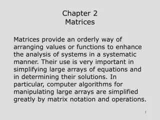
Chapter 2 Matrices
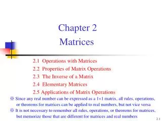
Linear Algebra. Chapter 2 Matrices. 2.1 Addition, Scalar Multiplication, and Multiplication of Matrices. a ij : the element of matrix A in row i and column j . For a square n n matrix A , the main diagonal is:. Definition

Chapter 2 Matrices
E N D
Presentation Transcript
Linear Algebra Chapter 2Matrices
2.1 Addition, Scalar Multiplication, and Multiplication of Matrices • aij: the element of matrix A in row i and column j. • For a squarenn matrix A, the main diagonal is: Definition Two matrices are equal if they are of the same size and if their corresponding elements are equal. ( for every, for all) Thus A = B if aij = bij i, j.
Addition of Matrices Definition Let A and B be matrices of the same size. TheirsumA + B is the matrix obtained by adding together the corresponding elements of A and B. The matrix A + B will be of the same size as A and B. If A and B are not of the same size, they cannot be added, and we say that the sum does not exist.
Determine A + B and A + C, if the sum exist. Example 2 Solution (2) Because A is 2 3 matrix and C is a 2 2 matrix, there are not of the same size, A + C does not exist.
Example 3 Observe that A and 3A are both 2 3 matrices. Scalar Multiplication of matrices Definition Let A be a matrix and c be a scalar. The scalar multiple of A by c, denoted cA, is the matrix obtained by multiplying every element of A by c. The matrix cA will be the same size as A.
Example Negation and Subtraction Definition We now define subtraction of matrices in such a way that makes it compatible with addition, scalar multiplication, and negative. Let A – B = A + (–1)B
Multiplication of Matrices Definition Let the number of columns in a matrix A be the same as the number of rows in a matrix B. The product AB then exists. Let A: mn matrix, B: nk matrix, The product matrix C=ABhas elements C is a mk matrix. If the number of columns in A does not equal the number of row B, we say that the product does not exist.
Example 4 Sol. Note.In general, ABBA. BA and AC do not exist.
Example 6 Determine c23. Let C = AB, Example 5 Determine AB.
A m r Example 7 If A is a 5 6 matrix and B is an 6 7 matrix. Because A has six columns and B has six rows. Thus AB exits. And AB will be a 5 7 matrix. Size of a Product Matrix If A is an m r matrix and B is an r n matrix, then AB will be an m n matrix. B = AB r n m n
Special Matrices Definition A zero matrix is a matrix in which all the elements are zeros. A diagonal matrix is a square matrix in which all the elements not on the main diagonal are zeros. An identity matrix is a diagonal matrix in which every diagonal element is 1.
Example 8 Theorem 2.1 Let A be m n matrix and Omn be the zero m n matrix. Let B be an n n square matrix. On and In be the zero and identity n n matrices. Then A + Omn = Omn + A = A BOn = OnB = On BIn = InB = B
Exercise 11 Let A be a matrix whose third row is all zeros. Let B be any matrix such that the product AB exists. Prove that the third row of AB is all zeros. Homework Solution
2.2 Algebraic Properties of Matrix Operations Theorem 2.2 -1 Let A, B, and C be matrices and a, b, and c be scalars. Assume that the size of the matrices are such that the operations can be performed. Properties of Matrix Addition and scalar Multiplication 1. A + B = B + A Commutative property of addition 2. A + (B + C) = (A + B) + C Associative property of addition 3. A + O = O + A = A (whereO is the appropriate zero matrix) 4. c(A + B) = cA + cB Distributive property of addition 5. (a + b)C = aC + bC Distributive property of addition 6. (ab)C = a(bC)
Theorem 2.2 -2 Let A, B, and C be matrices and a, b, and c be scalars. Assume that the size of the matrices are such that the operations can be performed. Properties of Matrix Multiplication 1. A(BC) = (AB)C Associative property of multiplication 2. A(B + C) = AB + AC Distributive property of multiplication 3. (A + B)C = AC + BCDistributive property of multiplication 4. AIn = InA = A (whereIn is the appropriate zero matrix) 5. c(AB) = (cA)B = A(cB) Note: AB BA in general. Multiplication of matrices is not commutative.
Example 1 Proof of Thm 2.2 (A+B=B+A) Consider the (i,j)th elements of matrices A+B and B+A: A+B=B+A
Compute ABC. Sol. (1) (AB)C (2) A(BC) Example 2 and 3 Which method is better? Count the number of multiplications. 26+32=12+6=18 32+22=6+4=10 A(BC) is better.
Arithmetic Operations If A is an m r matrix and B is r n matrix, the number of scalar multiplications involved in computing the product AB is mrn. Proof Consider the (i,j)th element of matrix AB: AB mn mrn ABC = D22 23 31 21 (1) (AB)C: 223+ 231=18 (2) A(BC): 231+ 221=10 better
Caution • In algebra we know that the following cancellation laws apply. • If ab = ac and a 0 then b = c. • If pq = 0 then p = 0 or q = 0. • However the corresponding results are not true for matrices. • AB = ACdoes not imply that B = C. • PQ = Odoes not imply that P = O or Q = O. Example
Powers of Matrices Definition If A is a square matrix, then Theorem 2.3 If A is an n n square matrix and r and s are nonnegative integers, then 1. ArAs = Ar+s. 2. (Ar)s = Ars. 3. A0 = In (by definition)
Example 5 Simplify the following matrix expression. Solution Example 4 Solution
Systems of Linear Equations A system of m linear equations in n variables as follows Let We can write the system of equations in the matrix form AX = B
Idempotent and Nilpotent Matrices(Exercise 30~36) Definition • A square matrix A is said to be idempotent if A2=A. • A square matrix A is said to nilpotent if there is a positive integer p such that Ap=0. The least integer p such that Ap=0 is called the degree of nilpotency of the matrix. Example
Exercise 8 Exercise 27 A : m r matrix, B:r n matrix, C: n s matrix. Derive formulas for the number of scalar multiplications involved in computing (AB)C and A(BC). A, B: diagonalmatrix of the same size, c: scalar Prove that A+B and cA are diagonal matrices. Homework • Exercise 2.2:6, 8, 11, 19, 27, 31, 33, 34, 35, 38
Exercise 31 Exercise 33 Determine b, c, and d such that is idempotent. Prove that if A and B are idempotent and AB=BA, then AB is idempotent. Homework
Example 1 2.3 Symmetric Matrices Definition Thetranspose of a matrix A, denoted At, is the matrix whose columns are the rows of the given matrix A.
Theorem 2.4 Properties of Transpose Let A and B be matrices and c be a scalar. Assume that the sizes of the matrices are such that the operations can be performed. 1. (A + B)t = At + Bt Transpose of a sum 2. (cA)t = cAt Transpose of a scalar multiple 3. (AB)t = BtAt Transpose of a product 4. (At)t = A
Theorem 2.4 Properties of Transpose Proof for 3. (AB)t= BtAt
match match Symmetric Matrix Definition A symmetric matrix is a matrix that is equal to its transpose. Example
If and only if • Let p and q be statements.Suppose that p implies q (if p then q), written p q,and that also q p, we say that“pif and only ifq” (iff )
Example 3 Let A and B be symmetric matrices of the same size. Prove that the product AB is symmetric if and only if AB = BA. Proof *We have to show (a) AB is symmetric AB = BA, and the converse, (b) AB is symmetric AB = BA. () Let AB be symmetric, then AB= (AB)tby definition of symmetric matrix = BtAt by Thm 2.4 (3) = BA since A and B are symmetric () Let AB = BA, then (AB)t = (BA)t = AtBt by Thm 2.4 (3) = AB since A and B are symmetric
Example 3 Let A be a symmetric matrix. Prove that A2 is symmetric. Proof
Example 4 Determine the trace of the matrix Solution We get Definition Let A be a square matrix. The trace of A, denoted tr(A) is the sum of the diagonal elements of A. Thus if A is an n n matrix. tr(A) = a11 + a22 + … + ann
Theorem 2.5 Properties of Trace Let A and B be matrices and c be a scalar. Assume that the sizes of the matrices are such that the operations can be performed. 1. tr(A + B) = tr(A) + tr(B) 2. tr(AB) = tr(BA) 3. tr(cA) = c tr (A) 4. tr(At) = tr(A) Proof of (1) Since the diagonal element of A + B are (a11+b11), (a22+b22), …, (ann+bnn), we get tr(A + B) = (a11 + b11) + (a22 + b22) + …+ (ann + bnn) = (a11 + a22 + … + ann) + (b11 + b22 + … + bnn) = tr(A) + tr(B).
The conjugate of a complex number z = a + bi isz = a- bi Matrices with Complex Elements The element of a matrix may be complex numbers. A complex number is of the form z = a + bi Where a and b are real numbers and a is called the real part and b the imaginary part of z.
Compute A + B, 2A, and AB. Example 6 Solution
Definition (i) The conjugate of a matrix A is denoted A and is obtained by taking the conjugate of each element of the matrix. (ii) The conjugate transpose of A is written and defined by A*=At. (iii) A square matrix C is said to be hermitian if C=C*. Example (i), (ii) Example (iii)
Exercise 11 A matrix A is said to be antisymmetric if A = -At. (a) give an example of an antisymmetric matrix.(b) Prove that an antisymmetric matrix is a square matrix having diagonal elements zero.(c) Prove that the sum of two antisymmetric matrices of the same size is an antisymmetric matrix. Homework • Exercise 2.3:2, 5, 11, 13, 15, 23
Exercise 13 Prove that any square matrix A can be decomposed into the sum of a symmetric matrix B and an antisymmetric matrix C: A = B+C. Homework (Find B: B = Bt, C: C = -Ct, such that A = B + C.) Solution (1) A = B + C A = Bt-Ct At= B -C (2) (1)+(2): A + At = 2B B= ½(A + At ) (1)-(2): A - At = 2C C= ½(A - At )
Example 1 Prove that the matrix has inverse Proof 2.4 The Inverse of a Matrix Definition Let A be an n n matrix. If a matrix B can be found such that AB = BA = In, then A is said to be invertible and B is called the inverse of A. If such a matrix B does not exist, then A has no inverse. (denote B = A-1, andA-k=(A-1)k ) Thus AB = BA = I2, proving that the matrix A has inverse B.
Thm2.2 Theorem 2.7 The inverse of an invertible matrix is unique. Proof Let B and C be inverses of A. Thus AB = BA = In, and AC = CA = In. Multiply both sides of the equation AB = In by C. C(AB) = CIn (CA)B = C InB = C B = C Thus an invertible matrix has only one inverse.
Since AA-1 =In, then A: an invertible nn matrixHow to find A-1? We shall find A-1 by finding X1, X2, …, Xn. Solve these systems by using Gauss-Jordan elimination: Note. [In:B] , A-1。
Gauss-Jordan Elimination for finding the Inverse of a Matrix Let A be an n n matrix. 1. Adjoin the identity n n matrix In to A to form the matrix [A : In]. 2. Compute the reduced echelon form of [A : In]. If the reduced echelon form is of the type [In : B], then B is the inverse of A. If the reduced echelon form is not of the type [In : B], in that the first n n submatrix is not In, then A has no inverse. An n n matrix A is invertible if and only if its reduced echelon form is In.
Determine the inverse of the matrix Example 2 Solution 隨堂作業:14
Example 3 Determine the inverse of the following matrix, if it exist. Solution There is no need to proceed further. The reduced echelon form cannot have a one in the (3, 3) location. The reduced echelon form cannot be of the form [In : B]. Thus A–1 does not exist.
Properties of Matrix Inverse Let A and B be invertible matrices and c a nonzero scalar, Then Proof 1. By definition, AA-1=A-1A=I.
Example 4 Solution
Theorem 2.8 Let AX = Y be a system of n linear equations in n variables. If A–1 exists, the solution is unique and is given by X = A–1Y. Proof (X = A–1Y is a solution.)Substitute X = A–1Y into the matrix equation. AX = A(A–1Y) = (AA–1)Y = InY = Y. (The solution is unique.) Let X1 be any solution, thus AX1 = Y. Multiplying both sides of this equation by A–1 gives A–1AX1= A–1YInX1 = A–1YX1 = A–1Y.
Solve the system of equations This system can be written in the following matrix form: If the matrix of coefficients is invertible, the unique solution is This inverse has already been found in Example 2. We get Example 5 Solution