Download
1 / 47
500 likes | 674 Vues
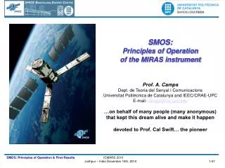
SMOS: Principles of Operation of the MIRAS instrument Prof. A. Camps Dept. de Teoria del Senyal i Comunicacions Universitat Politècnica de Catalunya and IEEC/CRAE-UPC E-mail: camps@tsc.upc.edu …on behalf of many people (many anonymous) that kept this dream alive and make it happen

E N D
SMOS: Principles of Operation of the MIRAS instrument Prof. A. Camps Dept. de Teoria del Senyal i Comunicacions Universitat Politècnica de Catalunya and IEEC/CRAE-UPC E-mail: camps@tsc.upc.edu …on behalf of many people (many anonymous) that kept this dream alive and make it happen devoted to Prof. Cal Swift… the pioneer
Outline of the presentation: • Basic principles • Imaging in Synthetic Aperture Radiometers: • 2.1. Synthetic Aperture Radiometers • 2.2. Image Reconstruction Algorithms: Ideal Case • The SMOS Mission • MIRAS instrument description • 4.1. Array topology • 4.2. Receivers’ architecture • 4.3. NIR architecture • 4.4. DIgital COrrelator System (DICOS) • 4.5. CAlibration System (CAS) • 5. Instrument Performance • 5.1. Angular Resolution • 5.2. Radiometric Performance: definition of terms • 5.3. Image Formation Through a Fourier Synthesis Process • 5.4. Imaging Modes: Dual-polarization and full-polarimetric • 6. Geolocalization: from director cosines grid to Earth reference frame grid • and Retrieval of Geophysical Parameters
b1(t) H1(f) Complex Correlator H2(f) b2(t) 1. Basic Principles • Spatial resolution is achieved by cross-correlating the signals collected by a number of antennas • Antennas can have a wide beam or a narrow one in one or two directions Channel 1 Channel 2 Baseline = antenna spacing normalized to the wavelength 2D Fourier Transform Ideal case: - Identical antenna patterns - Negligible spatial decorrelation - No antenna positioning errors
2. Imaging in Synthetic Aperture Radiometers 2.1. Synthetic Aperture Radiometers using Fourier Synthesis: Radioastronomy Earth Observation (concept proposed in 1983 by LeVine & Good) VLA, New Mexico, Socorro ESTAR (1 D Aperture Synthesis) NASA MIRAS (2 D Aperture Synthesis) ESA
Differences between radio-astronomy and Earth observation: • - Large antenna spacing • Very narrow field of view (FOV) • Obliquity factor (1/cos ) can be approximated by 1 • Antenna patterns are approximatedly constant (amplitude and phase) over the FOV • Typically quasi-point sources imaged over cold background • super-resolution image reconstruction algorithms can be used
. After the successful results ofESTAR radiometer (1988), theEuropean Space Agency starts in1993 the first feasibility studies to apply synthetic aperture microwave radiometry in two dimensions: .MIRAS concept is born: Microwave Imaging Radiometer by Aperture Synthesis .First studies (1993-95): led byMatra Marconi Space as the prime contractor .1995 Soil Moisture and Ocean Salinity Workshop (ESTEC, the Netherlands) Aperture Synthesis Microwave Radiometry is the only technique capable of measuring soil moisture and ocean salinity with enough accuracy and spatial resolution. SSS image derived from the ’“Electronically Steered Thinned Array Radiometer (ESTAR)”. Error = 0.3 psu (D. M. LeVine et al., NASA Goddard).
2.2. Image Reconstruction Algorithms: Ideal Case Antenna Positions Spatial frequencies (u,v) Periodic extension u v Overlapping of 1 alias Overlapping of 2 aliases Alias-free Field Of View (AF-FOV) 21 elements + 2 redundant elements/arm Antenna spacing d = 0.875 Hexagonal grid in (u,v) plane Nyquist criterion: d<
In SMOS the “alias-free FOV” can be enlargedsince part of the alias images are the “cold” sky (including the galaxy!) TB image limited by Earth replicas Iso-incidence angle contours Extension of Alias-Free FOV • Pixel axial ratio a/b • Spatial resolution defined as geometric mean of axes
3. The SMOS Mission • SMOS is a challenge: • Particularities of 2D aperture synthesis radiometers: • 1) New type of instrument: • - Review of the fundamental equation • - Detail error model & error correction (calibration) algorithms • - Image reconstruction algorithms • 2) New type of observations: • Multi-look and multi-angleobservations: • . different pixel size and orientation • . different noise and precision for each pixel • -Polarization mixing: • . Earth reference frame antenna reference frame • 3) New L-band and multiangular ocean • and soil emission models : • - Wide range of incidence angles (0º-60º) • 4) New geophysical parameter retrieval algorithms • taking into account issues 1, 2 and 3 above
SMOS Mission: SMOS Proba-2 • Scientific measurements require a • Sun-synchronous, • dawn/dusk, and • quasi circular orbit. • Orbital parameters: • Mean altitude = 755.5 km • Eccentricity = 0.001165 • Mean inclination = 98.416º • Local Time Asc. Node =6 AM • Argument of Perigee = 90º • Mean Anomaly = 306.3º • Note: The SUN is nearly always visible (97 % of the time) !!! Transformed SS-19 missile
4. MIRAS instrument description 4.1. Array topology • 69 antenna elements (LICEF) • Equally distributed over the 3 arms and hub • The acquired signal is transmitted to a central correlator unit, which computes the complex cross-correlations of all signal pairs.
[credits EADS-CASA] MIRAS consists of a central structure (hub) with 15 elements, and 3 deployable arms, each one having 3 segments with 6 antennas each.
1BIT ADC SLOPE CORR. IF FILTER IF AMPs ATTEN 1404-1423 MHz DICOS DI I ANTENNA SWITCH ISOL LNA BPF RFAMP MIXER TI H V 8-27 MHz C U TQ TRF Q DICOS DQ VCO SYNTH MAIN PATH GAIN = 100 dB 1BIT ADC SLOPE CORR. IF FILTER IF AMPs ATTEN PMS PATH GAIN = 65 dB 1396 MHz REF 55.84 MHz PMS 4.2. Receivers’ architecture: • PMS acts as a total Power Radiometer in each LICEF • Needed to denormalize the “normalized” correlations (1 bit/2 level)
LICEF: the LIght and Cost Effective Front-end [credits MIER Comunicaciones]
4.3. NIR architecture • TheNoise Injection Radiometer (NIR)is fully polarimetric and operates at 1.4 GHz • 3 NIRs in the hub for redundancy. • Functions: • precise measurement of Vpq(0,0) = TApq for mean value of TBpq(,) image. • measurement of noise temperature level of the reference noise source of Calibration Subsystem (CAS) absolute amplitude reference 1st LICEF unit (V-pol) Correlated noise inputs (from Noise Distribution Network) allow phase/amplitude calibration of receivers as LICEFs & for 3rd and 4th Stokes parameters measurements Controller unit (switches, noise injection...) 2nd LICEF unit (H-pol) [credits TKK]
SMOS NIR: [Colliander et al., 2005] Normal mode of operation: Calibrating internal noise source mode: known (cold sky) ? T NA + TA = TREF + TNR T NA + TA = TU [credits HUT]
4.4. DIgital COrrelator System (DICOS) 1 bit ADC (comparator) in each LICEF Correlator = = NOT-XOR + up-counter Digital signals from each LICEF are transmitted to DICOS to compute the complex cross-correlations of all signal pairs.
Lower half: II-correlations: Nr,Nc Zr r Vr • Upper half: IQ-correlations: Ni,Nc Zi i Vi • Diagonal: IQ-correlations of same • element (q: quadrature errors) • Correlations of I and Q signals with 0’s and 1’s • to compensate comparators’ threshold errors • Correlations of 0’s and 0’s and 1’s and 1’s = Ncmax • NCmax = 65437 for dual-pol mode (= fCLK · int) • NCmax = 43625 for full-pol mode • Total number of products: • 2556 correlations Ik-Ij • 2556 correlations Ik-Qj • 72 correlations Ik-Qk • 72 correlations I-0 • 72 correlations Q-0 • 72 correlations I-1 • 48 correlations Q-1 • 36 control correlations between 1 and 0 channels (4 for each ASIC)
CCU: the Correlator and Control Unit [credits EADS-CASA]
4.5. CAlibration System (CAS) Noise sources needed to calibrate the instrument. HUB ARMS
Centralized and distributed calibration • Correlated noise is injected to the receivers in two steps: • first the “even” sources and then using the “odd” ones Overlapping between elements (phase & amplitude tracking along the arms) Centralized Calibration (separable & non-separable errors can be corrected) Distributed Calibration (only separable errors can be corrected) These receivers belong to the NIR (□: H-channel) and do not form additional baselines Overlapping between elements (phase & amplitude tracking among arms)
OVERALL SEGMENT ARCHITECTURE [credits EADS-CASA]
6 LICEF / segment [credits EADS-CASA]
MOHA [credits EADS-CASA]
CAS [credits EADS-CASA]
CMN [credits EADS-CASA]
5. Instrument Performance 5.1. Angular Resolution • The “ideal” brightness temperature image is formed by an inverse • (discrete) Fourier transform of the measured visibility samples (B = 0): Equivalent Array Factor: same response as for an array of elements at (u,v) positions (except for the |(.)|2) • The retrieved image is the 2D convolution of the original T(,) image • with the instrument’s impulse response or equivalent array factor:
Response with rectangular window Response with Blackmann window (rotational symmetry) • W(umn,vmn): window • to weight the visibility • samples: • reduces side lobes • widens main lobe • increases main beam • efficiency (MBE)
Radiometric Sensitivity over ocean Dashed lines. Theoretical formula: Cut for =0 [credits I. Corbella]
Scene Bias < 0.1 K Galaxy Alias Moon Cosmic Background Radiation at 3.3 K Accuracy < 0.5 K Sun Alias Galaxy (yellowish) Galactic radio-source (TBC) [credits DEIMOS]
Singularity in the transformation antenna to Earth reference frame (dual-pol mode) Incidence angle dependence • 45 deg singularity discarded • All points with the same incidence angle averaged Fresnel [credits I. Corbella]
5.3. Image Formation Through a Fourier Synthesis Process • Even in the ideal case: • Antenna spacing > /3 aliasing • Gibbs phenomenon near the sharp transitions (mainly alias borders) • In the real case: • - Antenna patterns are different • Receivers’ frequency responses are different ( FWF different) • Antenna positioning errors (u,v,w)real different from (u,v,0)ideal IHFFT cannot be used as image reconstruction method More sophisticated algorithms must be devised But it will be good that the second ones tend to IHFFT in ideal conditions • … and obviously instrumental errors must be calibrated first!
Aperture Synthesis Radiometer: 2 step calibration Real Aperture Radiometer: 1 step calibration TB imaging pixel by pixel through antenna scan: TB imaging in a single snap-shot (1 integration time = 1.2 s / polarization in dual-pol): • Absolute calibration • External references: • Thot, Tcold • 1) Receivers relative calibration (image “contrast”) • - Error model (distorsions, artifacts, blurring…) • Internal references (Tcorr, Tuncorr,…) *** Imaging by (e.g.) conical scan *** *** Image Reconstruction Algorithm *** • 2) Absolute Calibration (image accuracy) • External references (FTT, OTT…) • Thot/Tcold, ground truth, external calibration…
Items that need calibration: NIR Gain and Offset PMS gain and offset (receiver and baseline amplitude errors) Fringe-washing function FWF (amplitude and phase errors) Noise that is injected to receivers during calibration Correlator Offsets Types of Calibration: Internal: injection of correlated or uncorrelated noise to the receivers External: observation of known target: NIR absolute calibration Flat-Target Transformation: to calibrate antenna pattern errors CAS Calibration: performed by NIR during internal calibration Correlator Calibration: injecting known signals Calibration Concept: Brief sketch
a. MIRAS internal calibration Instrumental errors correction: set of measurements and mathematical relations to remove instrumental errors INTERNAL INSTRUMENT CALIBRATION Error model • Characterizes the instrument behavior independently of the input signal. • It can be characterized by suitable internal known signals injected at its input: correlated/uncorrelated and hot/cold noise injection.
MIRAS Internal calibration PMS gain PMS offset Correlation amplitude (*) Calibrated visibility: (*)
Formulation of the Problem: Instrument Equation After Internal Calibration To be corrected using the Flat Target Response [credits I. Corbella]
The Flat Target Response: • The Flat Target Response is defined by: defining: Then the differential visibilities to be processed are:
External calibration • Once in a month (every week during commissioning) the platform rotates to point to the cold sky • External calibration is used to correct for elements not included in internal calibration: switch and antenna losses • Also the Noise Injection Radiometer (NIR) is calibrated and the Flat Target Response (FTR) measured HERE IT GOES THE ANIMATION. T_X_skylook2.gif HERE IT GOES THE ANIMATION. T_Y_skylook2.gif Tx and Ty while satellite is turning up [credits I. Corbella]
5.4. Imaging Modes: Dual-polarization and full-polarimetric Dual-polarization radiometer: MIRAS has dual-pol antennas, but only one receiver polarizations have to be measured sequentially, with an integration time of 1.2 s each [credits M. Martin-Neira]
Full-polarimetric mode:(selected as operational mode for SMOS) [credits M. Martin-Neira]
6. Geolocalization and Retrieval of Geophysical Parameters 6. Geolocalization: from director cosines grid to Earth reference frame grid • ISEAfamily of grids seem to be the best option for the SMOS Products, butEASE-Grid has come to be popular amongst many of the Earth Observation missions of the USA, namely AQUA (NASA/NASDA) and AQUARIUS (NASA), which are particularly interesting for comparison with the SMOS products. • Spatial partitioning of EASE-Grid is square-based and ISEA can be triangular, hexagonal or diamond-based: • - In its hexagonal form, ISEA has a higher degree of compactness, quantize the plane with the smallest average error and provides the greatest angular resolution. • ISEA hexagonal possesses uniform adjacency with its neighbors, unlike the square EASE-Grid. • Both grids have uniform alignment and are based on a spherical Earth assumption. • ISEA hexagonal at aperture 4 and resolution 9 (15km) is made up of 2,621,442 points and the EASE-Grid at 12km has 3,244,518 points. • EASE-Grid is congruent, whereas ISEA is not congruent, being impossible to decompose a hexagon into smaller hexagons or aggregate hexagons into larger ones. This would be a negative feature for real-time re-gridding, but in SMOS the grids will be pre-generated.
Auxiliary data Snap-shot 1 OS map (1 overpass) Spatio-temporal averaging Snap-shot 2 Multi-angular emission models Snap-shot 3 SM map (1 overpass) Snap-shot 4 L1 processor L2 processor L3 processor • Atmospheric and foreign sources corrections • Use of multiangular information: • 1. Th & Tv or Tx and Ty + Faraday and geometric rotations corrections: • Earth Antenna: retrieval in antenna ref frame, • Antenna Earth: retrieval in Earth ref frame, • 2. First Stokes parameter: I = Tx+Ty=Th+Tv. (invariant to rotations)
Sample SMOS data: Pixel in different positions of SMOS swath • OS retrieval: (pin 3) (pin 5)
40 km SMOS soil moisture [m3/m3] (a) Murrumbidgee catchment 1 km downscaled SMOS soil moisture [m3/m3] using MODIS VIS/IR data (b) MODIS NDVI [m3/m3] (c) MODIS LST [m3/m3] 60 km • Sample SMOS data over Australia: Murrumbidge catchement Sample results of the application of the downscaling algorithm to a SMOS image covering the Murrumbidgee catchment, South-Eastern Australia, on January 19, 2010 (6 am). First row: 40 km SMOS soil moisture [m3/m3] over Murrumbidgee (left), and zoom into Yanco site (right). Second row: 1 km downscaled soil moisture [m3/m3] over Murrumbidgee (left), and zoom into Yanco site (right). Dots indicate the location of the soil moisture permanent stations within the Murrumbidgee catchment used for validation purposes with colors representing their measurement at the exact SMOS acquisition time (only within Yanco site). Empty areas in the images correspond to non-retrieved soil moisture or clouds masking MODIS Ts measurements. (a) 60 x 60 km Yanco site in the Murrumbidgee catchment, South-Eastern Australia, (b) 1 km MODIS NDVI, and (c) and LST [K] on January 19, 2010.