Download
1 / 62
630 likes | 899 Vues
Chapter 19 Using Options for Risk Management. I. The Greeks II. Riskless Hedging III. Delta Hedging and Delta-Gamma Hedging IV. Position Deltas and Position Gammas V. Time Spreads VI. Caps, Floors, and Collars. The Greeks. 1 Theta is often expressed as a negative number.

E N D
Chapter 19Using Options for Risk Management I. The Greeks II. Riskless Hedging III. Delta Hedging and Delta-Gamma Hedging IV. Position Deltas and Position Gammas V. Time Spreads VI. Caps, Floors, and Collars
The Greeks 1 Theta is often expressed as a negative number
We Know that the Value of a Call Option Depends on the Values of: • Stock Price • Time to Expiration • Volatility • Riskless interest rate (generally assumed to be constant) • Dividend yield (generally assumed to be constant) • Strike Price (never changes)
Accordingly, as These Factors Change over time: • The value of the call option will change over time. • This is important for risk management because the composition of a “riskless” hedge must, therefore, change over time.
Some Intuition From Using a Taylor-Series Expansion • Given value at x0, we can use derivatives of function to approximate value of functionat x: f(x) = f(x0) + f ' (x0) (x-x0) + (1/2) f '' (x0)(x-x0)2 + ... • Incorporate curvature effects via Second-order Taylor series expansion of option price around the stock price (quadratic approximation): C(S + dS) = C(S) + (C/S) dS + (0.5) ∂2C/∂S2 (dS)2 = C(S) + DdS + 0.5 G (dS)2 • So, the change in the call price, given a change in S is: C(S + dS) - C(S) = DdS + 0.5 G (dS)2 + … dC = DdS + 0.5 G (dS)2 + …
Option price Slope = D B Stock price A Delta AKA: Hedge Ratio Delta (D) is the rate of change of the option price with respect to the underlying. (I.e., How does the option price change as the underlying price changes?)
Gamma Addresses Delta Hedging Errors Caused By Curvature Call price C’’ C’ C Stock price S S’
Example: • An investment bank has sold (for $300,000) a European call option on 100,000 shares of a non-dividend paying stock: i.e, • S0 = 49, K = 50, r = 5%, s = 20%, T = 20 weeks • The Black-Scholes value of the option is $240,000. • How does the investment bank hedge its risk?
Two Alternatives: • “Naked” position: Take no action (other than deep breath and hope for the best). Risk: Stock price is greater than $53 at expiration. • Covered position: Buy 100,000 shares today. Risk: Stock price is less than $46 at expiration.
Stop-Loss Strategy Which Involves: • Buying 100,000 shares as soon as price reaches $50. • Selling 100,000 shares as soon as price falls below $50. • NB: This deceptively simple hedging strategy does not work well. Main failure: Bid-Ask Spreads. (Think about “bid-ask bounce”)
Delta Hedging • This involves maintaining a “delta neutral” portfolio. • The delta of a European call on a non-dividend paying stock is N (d1). • The delta of a European call on a stock paying dividends at rate q is N (d1)e– qT. • The delta of a European put is on a non-dividend paying stock is: [N (d1) – 1]. • The delta of a European put on a stock paying dividends at rate q is e– qT[N (d1) – 1].
Delta Hedging, Cont. • N.B. The hedge position must be rebalanced “frequently.” (Delta Hedging is a concept born from Black-Scholes, I.e., in continuous time.) • Delta hedging a written option involves a “buy high, sell low” trading rule. (I.e., When S increases, so does Delta, and vice versa.) • Data from above: S0 = 49, K = 50, r = 0.05, s = 0.20, T = 20 weeks (0.3846) Option written on 100,000 shares, selling price: $300,000 Black-Scholes value of this option: $240,000
A Closer Look at Delta Hedging • Important: • Option on 100,000 shares • Volatility is assumed constant. • “Rebalancing” assumed weekly.
Aim of Delta Hedging: Keep Total Wealth Unchanged. Let’s look at the end of Week 9. • Value of written option at start: $240,000 (per B-S.) • Value of option at week 9 (s=20%): $414,500. • Option Position Loss: $(174,500). • Cash Position Change, (Measured by Cum. Cost: $2,557,800 – 4,000,500 = $(1,442,700). • Value of Shares held: • At start: 49 * 52,200 = $2,557,800 • At end of week 9: 53 * (67,400 + 11,300) = $4,171,100. • Increase of: $1,613,300. • Net: $1,613,300 – 1,442,700 – 174,500 = $(3,900).
More on Delta Hedging Delta is the (fractional) number of shares required to hedge one call. • Positions in the fractional shares and call have opposite signs. • For calls, delta lies between 0 and 1. • For puts, delta lies between –1 and 0. • Strictly speaking, the riskless hedge exists only for small changes in the stock price and over very small time intervals. • As time passes and/or the stock price changes, the D of the call changes (as measured by gamma). • As D changes, shares of stock must be bought or sold to maintain the riskless hedge.
Gamma • Gamma (G) is the rate of change of delta (D) with respect to the price of the underlying asset. • This G varies with respect to the stock price for a call or put option. (G reaches a maximum at the money). • As a rule, we would prefer to have a positive Gamma (more on this later…)
Interpretation of Gamma For a delta neutral portfolio, dP=Q dt + ½GdS2 dP dP dS dS Positive Gamma Negative Gamma
Position, or Portfolio, Deltas • The position delta determines how much a portfolio changes in value if the price of the underlying stock changes by a small amount. • The portfolio might consist of several puts and calls on the same stock, with different strikes and expiration dates, and also long and short positions in the stock itself. • The delta of one share of stock that is owned equals +1.0. The delta of a share of stock that is sold short is –1.0. Why?
Calculating a Position Delta • Assuming that each option covers one share of stock, the position delta is calculated as a weighted sum of individual deltas. That is, • where ni is the number of options of one particular type, or the number of shares of stock. • The sign of ni is positive if the options or stock is owned, and negative if the options have been written or the stock sold short. • The delta of the ith option or stock is given by Di.
An Example of a Position Delta Suppose you have positions in the following assets: Position and number of options or shares ni___ delta/unit Total Deltas=niDi long 300 shares +300 1.00 300.00 long 40 puts +40 -0.46 -18.40 short 150 calls -150 0.80 -120.00 long 62 calls +62 0.28 17.36 Dp = 178.96 This assumes that each option is on one share of stock
In this example, the position delta of 178.96 is positive. • This means that if the stock price were to increase by one dollar, the value of this portfolio would rise by $178.96. • If the stock price were to decline by one dollar, then the value of this portfolio would fall by $178.96. (Remember that this example assumes that the underlying asset of an option is one share of stock.) • Knowing your portfolio's position delta is as essential to intelligent option trading as knowing the profit diagrams of your portfolio.
Position Gammas Similar to position deltas, a position gamma is the weighted sum of the gammas of the elements of the portfolio: • where ni is the number of options of one particular type. The sign of ni is positive if the option is owned, and negative if the option has been written. • The gamma of the ith option is given by Gi. Note that the gamma of a stock is zero, because the delta of a stock is always equal to one.
Ideally, a delta neutral hedger would like to maintain a portfolio with a positive gamma. • Recall that the gamma of a call or a put are given by the same formula and that gammas cannot be negative. • However, a portfolio can have a positive or negative gamma. • It is important to note that a portfolio with a positive gamma increases in value if the underlying stock value changes. • Further, a portfolio with a negative gamma decreases in value if the underlying stock value changes.
Time Spreads, I. • Time spreads are also sometimes called calendar spreads or horizontal spreads. • Time spreads are identified by the ratio of options written and purchased. • To create a 1:1 time spread, the investor buys one option and sells one option. • The two options must either be both calls, or both puts, and share the same strike price on the same underlying asset. • However, unlike most of the option portfolios discussed previously, the time spread portfolio of options has options with different maturity dates.
Time Spreads, II. • The maximum profit on a time spread occurs when the stock price equals the strike price on the expiration date of the nearby call. • The short-term written option expires worthless, and the longer term option can be sold with some time value remaining. • An important risk to be kept in mind is that if the written, short-term option is in-the-money as its expiration date nears, it could be exercised early. • Thus, in-the-money time spreads using American options will often have to be closed out early in order to preclude this possibility.
Neutral Time Spreads • A neutral time spread is a strategy designed to capitalize on two options that are somehow “mis-priced” relative to each other. • The two options differ only in their times to expiration. • Usually the short-term option is written and the longer option is purchased. • The number of each option traded is designed to create a delta neutral portfolio.
Neutral Time Spreads, Example • Suppose the implied standard deviations of the two options were 0.4043 (for a September call), and 0.3262 (for a December call.) • Thus, assuming that the BSOPM is the proper pricing formula, the short-term call is overvalued relative to the December call. • Assume that the "true" volatility is 0.40/year. • Then, the hedge ratios of the two options are D = 0.4439 for the September call, and D = 0.5415 for the December call. • A delta neutral portfolio of these two options is: Dp = 0 = n1D1 + n2D2
Rearranging: • Using the above deltas, and denoting the September and December calls as assets 1 and 2, respectively: • Equation (19-6) says that to create a delta neutral position: 1.22 September calls should be sold for each December call purchased. • This allows the investor to arbitrage the relative mispricing of the two options, and not speculate on price movements.
Caveats • Of course, there are real risks and costs that must be included. • For example, we have ignored transactions costs. • In practice, the position will have to be closed out early if the options are in the money as September 21 nears, because the September call could be exercised early. • If they are exercised, the trader will bear additional transactions costs of having to purchase the stock and making delivery. In addition, there are rebalancing costs of trading options to maintain delta neutrality. For this reason, neutral hedgers prefer low gamma positions, if possible. • We assumed there are no ex-dividend dates between August 1 and September 21. Dividends would affect the computed deltas and also introduce early exercise risk. • We assumed constant interest rates and constant volatility. These also affect the computed deltas and indeed, may be the source of the apparent mispricing.
Caps • A cap is a purchased call option in which the underlying asset is an interest rate. • Note that a call on an interest rate is equivalent to a put on a debt instrument. • The interest rate cap is actually established when the interest rate call is combined with an existing floating rate loan. The call caps the interest that can be paid on the floating rate liability.
Buying a cap provides insurance against an interest rate increase that hurts the firm ΔV long call (at the money) Δr A rise in interest rates increases interest expense.
Buying a cap provides insurance against an interest rate increase that hurts the firm DV long call Δr resulting exposure The firm benefits from a decline in r, but has bought insurance to protect itself from a rise in r.
Caps • An interest rate call is purchased along with a variable rate loan to create the cap. The borrower then pays: if r < rc rc if r > rc • The interest rate call payments themselves are: (r - rc) (notional principal) (d/360) if r > rc 0 if r < rc where: rc is the cap rate (strike price), and d is the # of days in the settlement period.
Effective Interest Cost under a Cap Interest Expense r rc
An Example of a “Caplet” • Suppose the cap rate is 7.00%. • If: • the reference interest rate (3-month LIBOR) is 7.90% on the settlement date, • there are 90 days in the settlement period, • and, NP = $15,000,000. • Then, the payment is: (0.079 - 0.070) ($15,000,000) (90/360) = $33,750 • A cap is a portfolio of caplets, each having a different expiration (reset) date.
The Cap Premium • When purchased along with a floating rate loan, the cap premium is often amortized, and just added to the periodic interest rates. • Example. • A firm borrows $15,000,000 at LIBOR, with 8 semiannual payments. • A cap will cost $300,000. PV = -300,000, i = .035*, n = 8 => caplet PMT = $43,643. • This will add 43,643/15,000,000 = 29 basis points per semiannual payment = 58 bp per year to the loan • That is, the firm will pay LIBOR + 58bp, capped at 7.58% per annum.
Floors • An interest rate floor is a put on an interest rate ( = a call on a debt instrument). • Lenders, or institutions that own floating rate debt (an asset), purchase interest rate floors. • The floor is actually created when the interest rate put is combined with the floating rate asset. The put places a floor (a minimum) on how low the institution’s interest income can be.
Firm buys an at the money interest rate put DV Dr long put raw exposure Firm is exposed to the risk that interest rates will decline
The Interest Rate Floor is Insurance Against Declining Interest Rates DV Net Exposure Net Exposure Dr long put Raw Exposure Firm is exposed to the risk that interest rates will decline. Buying the interest rate put = buying insurance.
Floors • Combine a floating rate asset with a floor. The lender then receives: if r > rf rf if r < rf • The floor payments themselves are: (rf - r) (notional principal) (d/360) if r < rf 0 if r > rf where: rf is the floor rate (strike price), and d is the # of days in the settlement period.
Effective Interest Income with a Floor Interest Income r rF
Interest Rate Collars • A collar combines the purchase of a cap at a high strike price with the sale of a floor at a low strike price. • Frequently, the cost of the cap equals the selling price of the floor, so that a zero cost collar is “purchased”. • A collar allows a firm with a floating rate liability to insure itself from the undesired impact of an interest rate rise, but pays for it by giving up the benefits of a rate decline.
Interest Rate Collar Profit Long Call rc r rf Written put
Interest Rate Collar Profit r rc rf
Interest Rate Collar Profit r rc rf The underlying risk exposure is to rising interest rates
Interest Rate Collar: Profit r rc rf underlying risk exposure
Effective Interest Expense Under a Collar Interest Expense r rf rc
Interest Rate Corridors • Corridors are purchased by a firm with a floating rate liability. The firm buys an interest rate call with a (relatively) low strike price, and sells a cheaper one with a higher strike price. buy low rc cap (in-the-money) Profit r sell cheaper higher rc cap (out-of-the-money)