Efficient Parallel Sorting Algorithms: Bitonic Sort and Sample Sort Techniques
This document explores effective parallel sorting algorithms, focusing on Bitonic Sort and Sample Sort. Bitonic Sort utilizes a divide-and-conquer strategy, enabling processors to sort elements such that each processor's keys are larger than those on the previous processor. The communication between processors is minimized to pairs, enhancing efficiency. We also delve into Sample Sort, which involves collecting samples from each processor and using splitters for efficient data distribution. These algorithms are crucial for sorting large datasets across multiple processors.

Efficient Parallel Sorting Algorithms: Bitonic Sort and Sample Sort Techniques
E N D
Presentation Transcript
Parallel Sorting Sathish Vadhiyar
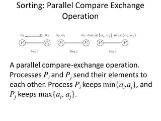
Sorting • Sorting n keys over p processors • Sort and move the keys to the appropriate processor so that every key on processor k is larger than every key on processor k-1 • The number of keys on any processor should not be larger than (n/p + thres) • Communication-intensive due to large migration of data between processors
Bitonic Sort • One of the traditional algorithms for parallel sorting • Follows a divide-and-conquer algorithm • Also has nice properties – only a pair of processors communicate at each stage • Can be mapped efficiently to hypercube and mesh networks
Bitonic Sequence • Rearranges a bitonic sequence into a sorted sequence • Bitonic sequence – sequence of elements (a0,a1,a2,…,an-1) such that • Or there exists a cyclic shift of indices satisfying the above • E.g.: (1,2,4,7,6,0) or (8,9,2,1,0,4) a0 an-1 ai
Using bitonic sequence for sorting • Let s = (a0,a1,…,an-1) be a bitonic sequence such that a0<=a1<=…<=an/2-1 and an/2>=an/2+1>=…>=an-1 • Consider S1 = (min(a0,an/2),min(a1,an/2+1),….,min(an/2-1,an-1)) and S2 = (max(a0,an/2),max(a1,an/2+1),….,max(an/2-1,an-1)) Both are bitonic sequences Every element of s1 is smaller than s2
Using bitonic sequence for sorting • Thus, initial problem of rearranging a bitonic sequence of size n is reduced to problem of rearranging two smaller bitonic sequences and concatenating the results • This operation of splitting is bitonic split • This is done recursively until the size is 1 at which point the sequence is sorted; number of splits is logn • This procedure of sorting a bitonic sequence using bitonic splits is called bitonic merge
Bitonic Merging Network 3 0 3 3 3 + + + + 5 3 0 5 5 + + + + 8 5 8 8 8 + + + + 9 8 5 0 9 + + + + 10 9 10 10 10 + + + + 12 10 9 12 12 + + + + 14 12 14 14 14 + + + + 20 14 12 9 0 + + + + 95 18 18 35 95 + + + + 90 20 20 23 90 + + + + 60 23 35 18 60 + + + + 40 35 23 20 40 + + + + 35 40 60 95 35 + + + + 23 60 40 90 23 + + + + 18 90 95 60 18 + + + + 0 95 90 40 20 + + + + Takes a bitonic sequence and outputs sorted order; contains logn columns A bitonic merging network with n inputs denoted as BM[n] +
Sorting unordered n elements • By repeatedly merging bitonic sequences of increasing length • An unsorted sequence can be viewed as a concactenation of bitonic sequences of size two • Each stage merges adjancent bitonic sequences into increasing and decreasing order • Forming a larger bitonic sequence BM[8] BM[4] BM[2] BM[16] + + BM[2] - + BM[2] BM[4] + - BM[2] - + BM[4] BM[2] BM[8] + + BM[2] - - BM[2] BM[4] + - BM[2] -
Bitonic Sort • Eventually obtain a bitonic sequence of size n which can be merged into a sorted sequence • Figure 9.8 in your book • Total number of stages, d(n) = d(n/2)+logn = O(log2n) • Total time complexity = O(nlog2n)
Parallel Bitonic SortMapping to a Hypercube • Imagine N processes (one element per process). • Each process id can be mapped to the corresponding node number of the hypercube. • Communications between processes for compare-exchange operations will always be neighborhood communications • In the ith step of the final stage, processes communicate along the (d-(i-1))th dimension • Figure 9.9 in the book
Parallel Bitonic SortMapping to a Mesh • Connectivity of a mesh is lower than that of hypercube • One mapping is row-major shuffled mapping • Processes that do frequent compare-exchanges are located closeby 5 1 4 0 7 3 6 2 13 9 12 8 15 11 14 10
Mesh.. • For example, processes that perform compare-exchange during every stage of bitonic sort are neighbors 5 1 4 0 7 3 6 2 13 9 12 8 15 11 14 10
Block of Elements per ProcessGeneral 3 0 3 3 3 + + + + 5 3 0 5 5 + + + + 8 5 8 8 8 + + + + 9 8 5 0 9 + + + + 10 9 10 10 10 + + + + 12 10 9 12 12 + + + + 14 12 14 14 14 + + + + 20 14 12 9 0 + + + + 95 18 18 35 95 + + + + 90 20 20 23 90 + + + + 60 23 35 18 60 + + + + 40 35 23 20 40 + + + + 35 40 60 95 35 + + + + 23 60 40 90 23 + + + + 18 90 95 60 18 + + + + 0 95 90 40 20 + + + +
General.. • For a given stage, a process communicates with only one other process • Communications are for only logP steps • In a given step i, the communicating process is determined by the ith bit
Drawbacks • Bitonic sort moves data between pairs of processes • Moves data O(logP) times • Bottleneck for large P
Sample Sort • A sample of data of size s is collected from each processor; then samples are combined on a single processor • The processor produces p-1 splitters from the sp-sized sample; broadcasts the splitters to others • Using the splitters, processors send each key to the correct final destination
Parallel Sorting by Regular Sampling (PSRS) • Each processor sorts its local data • Each processor selects a sample vector of size p-1; kth element is (n/p * (k+1)/p) • Samples are sent and merge-sorted on processor 0 • Processor 0 defines a vector of p-1 splitters starting from p/2 element; i.e., kth element is p(k+1/2); broadcasts to the other processors
PSRS • Each processor sends local data to correct destination processors based on splitters; all-to-all exchange • Each processor merges the data chunk it receives
Step 5 • Each processor finds where each of the p-1 pivots divides its list, using a binary search • i.e., finds the index of the largest element number larger than the jth pivot • At this point, each processor has p sorted sublists with the property that each element in sublist i is greater than each element in sublist i-1 in any processor
Step 6 • Each processor i performs a p-way merge-sort to merge the ith sublists of p processors
Analysis • The first phase of local sorting takes O((n/p)log(n/p)) • 2nd phase: • Sorting p(p-1) elements in processor 0 – O(p2logp2) • Each processor performs p-1 binary searches of n/p elements – plog(n/p) • 3rd phase: Each processor merges (p-1) sublists • Size of data merged by any processor is no more than 2n/p (proof) • Complexity of this merge sort 2(n/p)logp • Summing up: O((n/p)logn)
Analysis • 1st phase – no communication • 2nd phase – p(p-1) data collected; p-1 data broadcast • 3rd phase: Each processor sends (p-1) sublists to other p-1 processors; processors work on the sublists independently
Analysis Not scalable for large number of processors Merging of p(p-1) elements done on one processor; 16384 processors require 16 GB memory
Sorting by Random Sampling • An interesting alternative; random sample is flexible in size and collected randomly from each processor’s local data • Advantage • A random sampling can be retrieved before local sorting; overlap between sorting and splitter calculation
Radix Sort • During every step, the algorithm puts every key in a bucket corresponding to the value of some subset of the key’s bits • A k-bit radix sort looks at k bits every iteration • Easy to parallelize – assign some subset of buckets to each processor • Lad balance – assign variable number of buckets to each processor
Radix Sort – Load Balancing • Each processor counts how many of its keys will go to each bucket • Sum up these histograms with reductions • Once a processor receives this combined histogram, it can adaptively assign buckets
Radix Sort - Analysis • Requires multiple iterations of costly all-to-all • Cache efficiency is low – any given key can move to any bucket irrespective of the destination of the previously indexed key • Affects communication as well
Sources/References • On the versatility of parallel sorting by regular sampling. Li et al. Parallel Computing. 1993. • Parallel Sorting by regular sampling. Shi and Schaeffer. JPDC 1992. • Highly scalable parallel sorting. Solomonic and Kale. IPDPS 2010.
Bitonic Sort - Compare-splits • When dealing with a block of elements per process, instead of compare-exchange, use compare-split • i.e, each process sorts its local elementsl then each process in a pair sends all its elements to the receiving process • Both processes do the rearrangement with all the elements • The process then sends only the necessary elements in the rearranged order to the other process • Reduces data communication latencies
Block of elements and Compare Splits • Think of blocks as elements • Problem of sorting p blocks is identical to performing bitonic sort on the p blocks using compare-split operations • log2P steps • At the end, all n elements are sorted since compare-splits preserve the initial order in each block • n/p elements assigned to each process are sorted initially using a fast sequential algorithm
Block of Elements per ProcessHypercube and Mesh • Similar to one element per process case, but now we have p blocks of size n/p, and compare exchanges are replaced by compare-splits • Each compare-split takes O(n/p) computation and O(n/p) communication time • For hypercube, the complexity is: • O(n/p log(n/p)) for sorting • O(n/p log2p) for computation • O(n/p log2p) for communication
Histogram Sort • Another splitter-based method • Histogram also determines a set of p-1 splitters • It achieves this task by taking an iterative approach rather than one big sample • A processor broadcasts k (> p-1) initial splitter guesses called a probe • The initial guesses are spaced evenly over data range
Histogram SortSteps • Each processor sorts local data • Creates a histogram based on local data and splitter guesses • Reduction sums up histograms • A processor analyzes which splitter guesses were satisfactory (in terms of load) • If unsatisfactory splitters, the , processor broadcasts a new probe, go to step 2; else proceed to next steps
Histogram SortSteps • Each processor sends local data to appropriate processors – all-to-all exchange • Each processor merges the data chunk it receives Merits: • Only moves the actual data once • Deals with uneven distributions
Probe Determination • Should be efficient – done on one processor • The processor keeps track of bounds for all splitters • Ideal location of a splitter i is (i+1)n/p • When a histogram arrives, the splitter guesses are scanned
Probe Determination • A splitter can either • Be a success – its location is within some threshold of the ideal location • Or not – update the desired splitter to narrow the range for the next guess • Size of a generated probe depends on how many splitters are yet to be resolved • Any interval containing s unachieved splitters is subdivided with sxk/u guess where u is the total number of unachieved splitters and k is the number of newly generated splitters
Merging and all-to-all overlap • For merging p arrays at the end • Iterate through all arrays simultaneously • Merge using a binary tree • In the first case, we need all the arrays to have arrived • In the second case, we can start as soon as two arrays arrive • Hence this merging can be overlapped with all-to-all