Understanding MATLAB Functions and Arrays: A Guide to Manipulating Data Structures
This MATLAB lecture focuses on functions and structured data types, emphasizing the manipulation of one-dimensional and two-dimensional arrays. Learn how to efficiently use matrices, vectors, and text strings in various applications. Gain an understanding of operations like addition, subtraction, and division of matrices, along with the concepts of indexing and addressing elements within arrays. By the end of the lesson, you will be equipped to generate, manipulate, and work with arrays effectively, utilizing MATLAB's robust capabilities.

Understanding MATLAB Functions and Arrays: A Guide to Manipulating Data Structures
E N D
Presentation Transcript
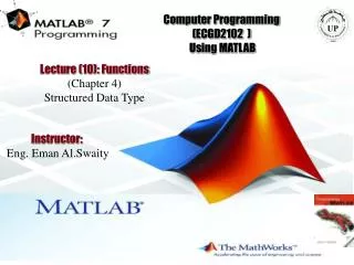
Computer Programming(ECGD2102 ) Using MATLAB Lecture (10): Functions (Chapter 4) Structured Data Type Instructor: Eng. Eman Al.Swaity
Objectives (CHAPTER (7):Plotting in MATLAB ) At the end of this lesson, you will be able to: • Use one and two dimensional arrays • Use text string. • Address elements in array. • Use arrays in applications
Introduction • One of MATLAB’s strengths lies in handling matrices and vectors very sufficiently. • MATLAB offers a variety of ways to generate data-array (vectors and matrices) • In most programming languages, variables that store multiple values are called arrays. Arrays can have many dimensions
Manipulating Matrices • In MATLAB, a matrix is a rectangular array of numbers. • One dimensional Array- Vector A one-dimensional array can be: Row Vectors:A row vector is an 1-by-n matrix so the number of rows is always one. The number of columns can be any integer value except one. Column Vectors: A column vector is an n-by-1 matrix so the number of columns is always one. The number of rows can be any integer value except one.
Manipulating Matrices • Scalars:Any single element or numerical value. Or said other way, any vector or matrix that has one row and one column. (Its size is equal to 1,1.)
Manipulating Matrices • Two Dimensional Array: Two-dimensional arrays can be thought of as a table. Here is an array with 4 rows and 5 columns: Square Matrices:Any matrix that has the number of rows equal to the number of columns (m = n).
Manipulating Matrices • Arrays of Text Strings In Section 4.2.1, we saw that a text string is a one-dimensional array whose elements are the individual characters in the string. Suppose we want to create an array whose elements are the days of the week. Now let's try to create a column array where each element of the array is one of the strings. With a column array, a new row is specified with a semicolon (; ).
Manipulating Matrices • Arrays of Text Strings the problem is : our strings are not the same length. In an array, each row must have the same number of Columns,
Vector & Matrix assignment • Vectors (arrays) are defined as >> v = [1, 2, 4, 5] >> w = [1; 2; 4; 5] • Matrices (2D arrays) defined similarly >> A = [1,2,3;4,-5,6;5,-6,7]
Operations on Matrices ADDITION AND SUBTRACTION The operations + (addition) and - (subtraction) can be used with arrays of identical size (the same number of rows and columns). The sum, or the difference of two arrays is obtained by adding, or subtracting, their corresponding elements. For Example if A and B are two arrays (for example 3 x 3 matrices), Then we can add or subtract them
Operations on Matrices ADDITION AND SUBTRACTION The figure shows how two differently sized vectors cannot be combined element-by-element, because there exist ambiguities as to how an operation is defined between a scalar and a "nothing".
Operations on Matrices MULTIPLICATION
Operations on Matrices MULTIPLICATION
Operations on Matrices DIVISION The division operation can be explained with the help of the identity matrix and the inverse operation. Identity matrix: The identity matrix is a square matrix in which the diagonal elements are 1's, and the rest of the elements are zeros. When the identity matrix multiplies another matrix (or vector), that matrix (or vector) is unchanged.
Operations on Matrices DIVISION determinant of a square matrix can be calculated with the inv(A) command
Operations on Matrices DIVISION Determinants: Determinant is a function associated with square matrices. determinant of a square matrix can be calculated with the det(A) command
Operations on Matrices DIVISION Array division: MATLAB has two types of array division, which are 1. Left division \ : The left division is used to solve the matrix equation AX = B. In this equation X and B are column vectors. This equation can be solved by multiplying on the left both sides by the inverse of A: In MATLAB the last equation can be written by using the left division character:
Operations on Matrices DIVISION
Operations on Matrices ELEMENT-BY-ELEMENT OPERATIONS
Operations on Matrices ELEMENT-BY-ELEMENT OPERATIONS
Array Addrissing (Indexing) Rows and columns of a matrix, indexing conventions, and the general form of indexing into a matrix.
Array Addrissing (Indexing) • Indexing using parentheses >> A(2,3) • Index submatrices using vectorsof row and column indices >> A([2 3],[1 2]) • Ordering of indices is important! >> B=A([3 2],[2 1]) >> B=[A(3,2),A(3,1);A(2,2);A(2,1)]
Array Addrissing (Indexing) • Index complete row or column using the colon operator • >> A(1,:) • Can also add limit index range • >> A(1:2,:) • >> A([1 2],:) • General notation for colon operator • >> v=1:5 • >> w=1:2:5
Array Addrissing (Indexing) Deleting Rows and Columns • You can delete rows and columns from a matrix using just a pair of square brackets >> X = A; Then, to delete the second column of X, use >>X(:,2) = [] This changes X to • If you delete a single element from a matrix, the result isn’t a matrix any more. So, expressions like >>X(1,2) = [] result in an error. However, using a single subscript deletes a single element,or sequence of elements, and reshapes the remaining elements into a row vector. So X(2:2:10) = [] results in
Array Addrissing (Indexing) Generating Vectors from functions x = zeros(1,3) x = 0 0 0 x = ones(1,3) x = 111 x = rand(1,3) x = 0.9501 0.2311 0.6068 • zeros(M,N) MxN matrix of zeros • ones(M,N) MxN matrix of ones • rand(M,N) MxN matrix of uniformly distributed random numbers on (0,1) • eye(m) reate a unit identity matrix
Array Addrissing (Indexing) Matrix and Mathematical Functions