Calculus
Learn the principles and techniques of calculus integration using MATLAB. Explore definite and indefinite integrals, integral pairs, closed-form integrals, and numerical integration with practical examples and applications.


Calculus
E N D
Presentation Transcript
Math Review with Matlab: Calculus Integration S. Awad, Ph.D. M. Corless, M.S.E.E. D. Cinpinski E.C.E. Department University of Michigan-Dearborn
Integration • Definite and Indefinite Integrals • Integral Pairs • Closed Form Integrals • Int Command • Closed Form Example • Multiple Independent Variable Example • Numerical Integration • Quad Command • Numerical Integration Example • Closed Form and Numerical Integration Example
Definite & Indefinite Integrals • A definite integral represents the area under a curve f(x) between the lower limit a and the upper limit b • An integral is considered to be indefinite if the upper and lower limits are not specified
Integral Pairs • Some indefinite integrals can be thought of as the inverse of differentiation • A few common integral pairs are shown below • Note that due to initial conditions, arbitrary integral pairs are not unique and may differ by a constant of integration, c
Closed Form Integrals • Closed form integrals are integrals which can be expressed as explicit functions • The integral pairs on the previous slide are examples of closed form integrals • Techniques such as partial fraction expansion, integration by parts, and integration by substitution can be used to express some integrals in closed form • It is not always possible to find the closed form for the integral of an arbitrary function
Evaluation of Definite Integral • If a closed form indefinite integral exists, it can be used to evaluate a definite integral over a region of integration • An integral from an arbitrary lower limit to a fixed upper limit is denoted as: • Thus definite integral from a lower limit a to an upper limit b can be evaluated using:
Int Command • The int command is used to solve integrals which can be expressed in closed form int(s) returns the indefinite integral of the symbolic variable s with respect to its default symbolic variable int(s,v) returns the indefinite integral of the symbolic variable s with respect to the symbolic variable v int(s,a,b) returns the definite integral of the symbolic variable s with respect its default symbolic variable from a to b int(s,v,a,b) returns the definite integral of the symbolic variable s with respect to the symbolic variable v from a to b
Closed Form Example • Given the function, f(x): 1) Use the int command to determine the Closed Form Indefinite Integral, F(x): 2) From the closed form integral, F(x), determine the definite integral of f(x) from 0 to p/2 3) Use the int command to directly determine the definite integral of f(x) from 0 to p/2 4) Determine and plot a function A(z) representing the general area under f from 0 to any arbitrary point z
Indefinite Closed Form • Matlab can be used to verify the integral pair shown on a previous slide • The integration variable parameter does not need to be specified since x is the only variable in the expression, hence it will be the default variable of integration » syms x » f=(sin(2*x)); » F=int(f) F = -1/2*cos(2*x)
Definite Integral Evaluation • The definite integral can be evaluated from the indefinite integral using the relationship: » Fb=subs(F,'x',pi/2) Fb = 0.5000 » Fa=subs(F,'x',0) Fa = -0.5000 » A_pidiv2 = Fb - Fa A_pidiv2 = 1
Matlab Direct Evaluation • Since f(x) has a closed form, the int command can be used to directly determine the definite integral » f=(sin(2*x)); » F_definite=int(f,0,pi/2) F_definite = 1
Area Under Curve • A general function, A(z), used to plot the area under the curve f(x) to an arbitrary point z can be determined as follows: » syms z » F_z = subs(F,x,z); » F_0 = subs(F,x,0); » A_z = F_z - F_0 A_z = -1/2*cos(2*z)+1/2 » A_z_pidiv2=subs(A_z,z,pi/2) A_z_pidiv2 = 1
Graphical Definite Integral • Area under f(x) from 0 to p/2 = 1 • Definite Integral Evaluation A(p/2) » subplot(2,1,1) » ezplot(f,0,pi) » grid on » subplot(2,1,2) » ezplot(A_z,0,pi) » grid on
Multiple Independent Variable Example • Given the function f(t,x,y): • Use Matlab to determine the closed form integrals with respect to the different independent variables: 1) Integrate f with respect to t : 2) Integrate f with respect to x : 3) Integrate f with respect to y :
Default Integration • Integrating with respect to the default independent variable will integrate with respect to x » syms t x y » f=sym('t + 2*t*x + 3*x*y*t'); » Fx = int(f) Fx = t*x+t*x^2+3/2*x^2*y*t
Other Independent Variables • Integration of f(t,x,y) with respect to t or y must be explicitly specified as an input argument to int » Ft=int(f,t) Ft = 1/2*t^2+t^2*x+3/2*x*y*t^2 » Fy=int(f,y) Fy = t*y+2*x*y*t+3/2*x*y^2*t
Numerical Integration • Some functions do not have closed form integrals • A definite integral can be numerically approximated provided that the function is defined over the region of interest • Numerical integration is performed by subdividing the integration region into very small regions, approximating the area in each region, and summing the areas • If as the length of the subintervals tends to 0 and the summation of areas tends to a unique limit, I, the definite integral over the interval is I
Quad Command • The quad command is used to numerically evaluate an integral Q = quad('f',a,b) approximates the integral of f(x) from a to b • 'f' is a string containing the name of an m-function to be integrated. Function f must return a vector of output values when given an input vector. • Q = Inf is returned if an excessive recursion level is reached, indicating a possibly singular integral. • Typically a new m-function will be created for f when numerically evaluating an integral
Numerical Integration Example • Given the function, f(x): • The definite integral, F: 1) Use the symbolic toolbox to verify that the f(x) does not have a closed form indefinite integral 2) Plot f(x) to ensure that the function is continuously defined over the integration region 3) Numerically integrate f(x) to determine F
No Closed Form • No closed form can be found using Matlab’s symbolic toolbox » f_sym = sin(x)*exp(-x^2); » int(f_sym) Warning: Explicit integral could not be found. > In C:\MATLABR11\toolbox\symbolic\@sym\int.m at line 58 ans = int(sin(x)*exp(-x^2),x)
Continuous Plot • A plot verified that f(x) is continuous over the integration region • Numerical integration is possible » ezplot(f_sym) » grid on
Numerical Integration • Must numerically evaluate the integral using the quad command which requires a function as an input • Create a new m-function describing the function: • The function must return a vector so be sure to use .* and .^ notations where appropriate function f = f_sin_exp_sqr( x ) f=sin(x).*exp(-x.^2);
Numerical Integration • Use the quad command to perform the numerical integration and evaluate the definite integral » F_num_int = quad('f_sin_exp_sqr',0,pi/2) F_num_int = 0.4024
Closed Form and Numerical Integration Example • Given the function f(x): • The definite integral, F: 1) Plot f(x) to ensure that the function is continuously defined over the integration region 2) Use the symbolic toolbox to evaluate the definite integral 3) Numerically integrate f(x) to determine the definite integral
Continuous Plot • Use ezplot to plot the function • Verified continuous from x=0 to x=4 » syms x » f_sym=exp(x)+atan(x); » ezplot(f_sym) » grid on
Symbolic Expression Symbolic Evaluation • Use the symbolic toolbox int command to evaluate definite integral from the closed form integral » defint_sym=int(f_sym,0,4) F_sym = exp(4)+4*atan(4)-1/2*log(17)-1 » defint_dbl=double(F_sym) defint_dbl = 57.4848
Numerical Evaluation • Create a new m-function to represent f(x): function f = f_exp_atan( x ) f=exp(x)+atan(x); • Use quad command to numerically evaluate the definite integral and verifythe previous symbolic result » defint_numint=quad('f_exp_atan',0,4) defint_numint = 57.4850 • Small difference to numerical approximation
Summary • Definite integrals are evaluated over a continuous interval and result in a number • Closed form indefinite integral functions exist for some functions independent of the integration limits • The definite integrals can be evaluated from the closed form indefinite integral if it exists • If a closed form indefinite integral does not exist, the definite integral of continuous functions can still be numerically approximated