Download
1 / 52
520 likes | 630 Vues
. ECEN 5341/4341 March 3,2014 Chapter 10. RF Models Start with simple plane wave models Progress to figures of revolution Numerical Approaches . Antennas. Near Field Far Field Transition Range from Short Dipole = λ /2 π. Some Basic Definitions.

E N D
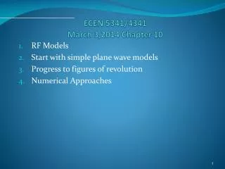
. ECEN 5341/4341March 3,2014 Chapter 10 RF Models Start with simple plane wave models Progress to figures of revolution Numerical Approaches
Antennas • Near Field • Far Field • Transition Range from • Short Dipole = λ/2π
Some Basic Definitions • 1 Specific Absorption Rate (SAR) in W/kg Where σ is the conductivity in S/m ρ is the density in kg/m3 and E is the electric field V/m • For short pulses • Where c is the specific heat capacity in J/kg oC • ΔT is the change in temperature • Δt is the length of the pulse
Thermal Relaxation Times • 1. For a short pulse in a Sphere • Where a is the radius and is the thermal diffusivity • And where k’ is the thermal conductivity. • Note for a long thin plate we get much faster thermal relaxation times as the surface to volume ratio increases as 1/t where t is the thickness.
Thermal vs. Non-thermal Biological Effects • 1 Temperature is a convenient way to define a distribution functions. The only case when you have a non-thermal system is when you have only one particle or one state. • 2. The common Maxwell Boltzmann distribution is given by 3 Another common distribution function is a Fermi-Dirac 4. Different temperatures for electrons and lattice.
Plane Waves • 1 This works for R/λ>> 1 • 2 Important parameters are f, polarization, angle of incidence,σ, and ε • 3 At normal incidence reflection coefficient • Where η1, η2 are impedances • The transmission coefficient is given by Going from 1 to 2. • The power reflected is given by Г2
Reflection as a Function of Angle and PolarizationFrom a Tissue Interface
Numerical Models • 1 Quasi-static < 30 to 40Mhz • 2 Method of Moments, MoM • 3. Finite Element, FEM • 4. Finite Difference Time Domain, FDTD
3D Impedance Models • 1. Assumes the dimensions are small compared to the wave length so that everything is at the same time. • zxzz • Zy
Volume Integral Method of Moments, VMoM • 1 Transforms Integral Equations into a matrix equations using the volume equivalence principle • 2 Break into N simple cells • 3. Satisfy the Boundary Conditions • 4. Get full matrices • 5. Takes lots of memory.
Finite Element Method FEM • 1. This has not been used much for biological estimates of the fields in humans • 2. It grows with the number of elements as N • 3. The choice of the elements and their shape is important. • 4. Use to form a system of linear equations. • 5. Satisfy the boundary conditions.
Finite Difference Time Domain • 1. Establish values of σ and ε for each cell • 2. Include the source. • 3. The boundary conditions are generated from the curl equations. • 4. Establish the E,H, about the unit cell then evaluate the values at alternate half time steps • 5. This calculation grows linearly with N • 6. This can be fast even for N = 106 • 7. This is the most commonly used approach.
Frequency –Dependent FDTD • 1 Used for short pluses and wide band where ε and σ vary with frequency. • 2 Two approaches • A. convert ε and σ to the time domain • B. Add the differential equation for displacement vector D Solve the equations simultaneously
Current Densities in the Body from the Magnetic Fields of an Electric Blanket
Current Densities in the Body from the Magnetic Fields of an Electric Blanket
Current Densities in the Body from the Magnetic Fields of an Electric Blanket
Cubic Cell Mode. • 1
Average SAR vs Frequency at10W/m2 and 80MHz Vertical Polarization