Econometric Analysis of Panel Data
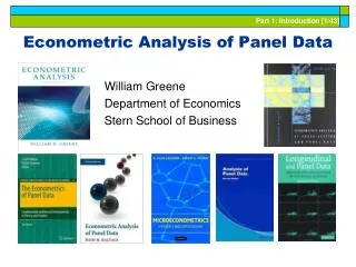
Econometric Analysis of Panel Data. William Greene Department of Economics Stern School of Business. Panel Data Modeling. Outcome(s) y i Model specification: Behavioral description Observation mechanism: Horizontal and time

Econometric Analysis of Panel Data
E N D
Presentation Transcript
Econometric Analysis of Panel Data William Greene Department of Economics Stern School of Business
Panel Data Modeling • Outcome(s) yi • Model specification: Behavioral description • Observation mechanism: Horizontal and time • Common effects built explicitly into the model: Observed and unobserved • Research Community: • Economics, political science, sociology: longitudinal, • Transport, marketing: stated choice experiments • Health: repeated measures, mixed models • Urban & regional economics: hierarchical models
Benefits of Panel Data • Time and individual variation in behavior unobservable in cross sections or aggregate time series • Observable and unobservable individual heterogeneity • Rich hierarchical structures • More complicated models • Features that cannot be modeled with only cross section or aggregate time series data alone • Dynamics in economic behavior
Panel Data Sets • Longitudinal data – ‘short panels’ • National longitudinal survey of youth (NLS) • British household panel survey (BHPS) • Panel Study of Income Dynamics (PSID) • German Socioeconomic Panel (GSOEP) • Medical Expenditure Panel Survey (MEPS) • Household income and labor dynamics (HILDA, Australia) • Cross section time series – ‘long panels’ • Grunfeld’s investment data • Penn world tables • Financial data by firm, year – ‘huge panels’ • rit – rft = i(rmt - rft) + εit, i = 1,…,many; t=1,…many • Exchange rate data, essentially infinite T, large N • Effects: i= + vi
Panel Data Sets • Longitudinal data – ‘short panels’ • National longitudinal survey of youth (NLS) • British household panel survey (BHPS) • Panel Study of Income Dynamics (PSID) • German Socioeconomic Panel (GSOEP) • Medical Expenditure Panel Survey (MEPS) • Household income and labor dynamics (HILDA, Australia) • Cross section time series – ‘long panels’ • Grunfeld’s investment data • Penn world tables • Financial data by firm, year – ‘huge panels’ • rit – rft = i(rmt - rft) + εit, i = 1,…,many; t=1,…many • Exchange rate data, essentially infinite T, large N • Effects: i= + vi
Panel Data Sets • Longitudinal data – ‘short panels’ • National longitudinal survey of youth (NLS) • British household panel survey (BHPS) • Panel Study of Income Dynamics (PSID) • German Socioeconomic Panel (GSOEP) • Medical Expenditure Panel Survey (MEPS) • Household income and labor dynamics (HILDA, Australia) • Cross section time series – ‘long panels’ • Grunfeld’s investment data • Penn world tables • Financial data by firm, year – ‘huge panels’ • rit – rft = i(rmt - rft) + εit, i = 1,…,many; t=1,…many • Exchange rate data, essentially infinite T, large N • Effects: i= + vi
Panel Data • Rotating panels: Spanish household survey • Spanish income/savings study • Efficiency analysis: “Efficiency measurement in rotating panel data,” Heshmati, A, Applied Economics, 30, 1998, pp. 919-930 • U.S. Survey of Income and Program Participation (SIPP) • Pseudo panel: Time series of (different) cross sections. E.g., Yearly UK Family Expenditure Survey; 7,000+ different households. What can we learn from these? • Hierarchical (nested) data sets: Student outcome, by year, district, school, teacher
SIPP Rotating Panel The lessons learned from ISDP were incorporated into the initial design of SIPP, which was used for the first 10 years of the survey. The original design of SIPP called for a nationally representative sample of individuals 15 years of age and older to be selected in households in the civilian noninstitutionalized population. Those individuals, along with others who subsequently lived with them, were to be interviewed once every 4 months over a 32-month period. To ease field procedures and spread the work evenly over the 4-month reference period for the interviewers, the Census Bureau randomly divided each panel into four rotation groups. Each rotation group was interviewed in a separate month. Four rotation groups thus constituted one cycle, called a wave, of interviewing for the entire panel. At each interview, respondents were asked to provide information covering the 4 months since the previous interview. The 4-month span was the reference period for the interview. The first sample, the 1984 Panel, began interviews in October 1983 with sample members in 19,878 households. The second sample, the 1985 Panel, began in February 1985. Subsequent panels began in February of each calendar year, resulting in concurrent administration of the survey in multiple panels. The original goal was to have each panel cover eight waves. However, a number of panels were terminated early because of insufficient funding. For example, the 1988 Panel had six waves; the 1989 Panel, part of which was folded into the 1990 Panel, was halted after three waves. In addition, the intent was for each SIPP panel to have an initial sample size of 20,000 households. That target was rarely achieved; again, budget issues were usually the reason. The 1996 redesign (discussed below) entailed a number of important changes. First, the 1996 Panel spans 4 years and encompasses 12 waves. The redesign has abandoned the overlapping panel structure of the earlier SIPP, but sample size has been substantially increased: the 1996 Panel had an initial sample size of 40,188 households.
Panel Data • Rotating panels: Spanish household survey • Spanish income/savings study • Efficiency analysis: “Efficiency measurement in rotating panel data,” Heshmati, A, Applied Economics, 30, 1998, pp. 919-930 • U.S. Survey of Income and Program Participation (SIPP) • Pseudo panel: Time series of (different) cross sections. E.g., Yearly UK Family Expenditure Survey; 7,000+ different households. What can we learn from these? • Hierarchical (nested) data sets: Student outcome, by year, district, school, teacher
Panel Data • Rotating panels: Spanish household survey • Spanish income/savings study • Efficiency analysis: “Efficiency measurement in rotating panel data,” Heshmati, A, Applied Economics, 30, 1998, pp. 919-930 • U.S. Survey of Income and Program Participation (SIPP) • Pseudo panel: Time series of (different) cohort cross sections. E.g., Yearly UK Family Expenditure Survey; 7,000+ different households. • Hierarchical (nested) data sets: Student outcome, by year, district, school, teacher
Nested Panel Data • Antweiler, W., “Nested Random Effects…” Journal of Econometrics, 101, 2001, 295-313 c s t
Cornwell and Rupert Data Cornwell and Rupert Returns to Schooling Data, 595 Individuals, 7 Years(Extracted from NLSY.) Variables in the file are EXP = work experienceWKS = weeks workedOCC = occupation, 1 if blue collar, IND = 1 if manufacturing industrySOUTH = 1 if resides in southSMSA = 1 if resides in a city (SMSA)MS = 1 if marriedFEM = 1 if femaleUNION = 1 if wage set by union contractED = years of educationLWAGE = log of wage = dependent variable in regressions These data were analyzed in Cornwell, C. and Rupert, P., "Efficient Estimation with Panel Data: An Empirical Comparison of Instrumental Variable Estimators," Journal of Applied Econometrics, 3, 1988, pp. 149-155. See Baltagi, page 122 for further analysis. The data were downloaded from the website for Baltagi's text.
Application: Health Care Panel Data German Health Care Usage Data, 7,293 Individuals, Varying Numbers of PeriodsVariables in the file areData downloaded from Journal of Applied Econometrics Archive. This is an unbalanced panel. They can be used for regression, count models, binary choice, ordered choice, and bivariate binary choice. This is a large data set. There are altogether 27,326 observations. The number of observations ranges from 1 to 7. (Frequencies are: 1=1525, 2=1079, 3=825, 4=926, 5=1051, 6=1000, 7=887). Note, the variable NUMOBS below tells how many observations there are for each person. This variable is repeated in each row of the data for the person. DOCTOR = 1(Number of doctor visits > 0) HOSPITAL = 1(Number of hospital visits > 0) HSAT = health satisfaction, coded 0 (low) - 10 (high) DOCVIS = number of doctor visits in last three months HOSPVIS = number of hospital visits in last calendar yearPUBLIC = insured in public health insurance = 1; otherwise = 0 ADDON = insured by add-on insurance = 1; otherswise = 0 HHNINC = household nominal monthly net income in German marks / 10000.HHKIDS = children under age 16 in the household = 1; otherwise = 0 EDUC = years of schooling AGE = age in years MARRIED = marital status
Econometric Analysis of Panel Data Overview
Panel Data Econometrics This is an intermediate level, Ph.D. course in the area of Applied Econometrics dealing with Panel Data. The range of topics covered in the course will span a large part of econometrics generally, though we are particularly interested in those techniques as they are adapted to the analysis of 'panel' or 'longitudinal' data sets. Topics to be studied include specification, estimation, and inference in the context of models that include individual (firm, person, etc.) effects.
Why a Course on ‘Panel Data?’ • Microeconometrics and applications – contemporary broad field in economics/econometrics • Behavioral modeling • Individual choice and response • A platform for surveying econometric models and methods – most of the field • Various types • Recent developments
Prerequisites • Econometrics I or equivalent Ph.D. level introduction to econometrics • Mathematical statistics • Matrix algebra We will do some proofs and derivations. We will examine many empirical applications. You will apply the tools developed in the course.
Text Readings • Baltagi (2008); Main text: read chapters 1,2 • Greene (2012); Recommended: read chapters 1,2,8,11,13 • Wooldridge (2010); Suggested: read chapters 1,2,4,10,11 • Cameron and Trivedi (2005); Very interesting: Microeconometrics • Matyas and Sevestre (2008); Recent survey. Contributed papers. • Hsiao(2003); Alternative to Baltagi • Frees (2004); Applications from many areas.
Course Applications • Problem sets • Panel data sets: See the course website • Software: NLOGIT Version 5.0 • Other ‘packages:’ Stata, SAS, EViews • Programming environments: R, Matlab, Gauss, Mathematica • We will not use class time for software instruction • ‘Lab’ work • Problem sets • Questions and review as requested
http://people.stern.nyu.edu/wgreene/Econometrics/PanelDataEconometrics.htmhttp://people.stern.nyu.edu/wgreene/Econometrics/PanelDataEconometrics.htm
Other Data Sets Data sets for Econometric Analysis Data sets for Baltagi’s Text
Where Do We Go From Here? • Review of familiar classical procedures • Fundamental, familiar regression extensions; common effects models • Endogeneity, instrumental variables, GMM estimation • Dynamic models • Models of heterogeneity • Nonlinear models that carry forward the features of the linear, static and dynamic common effects models • Recent developments in non- and semiparametric approaches
Econometric Models • Linear; static and dynamic • Discrete choice • Censoring and truncation • Structural models and demand systems • Time series models
Estimation Methods and Applications • Least squares etc. – OLS, GLS, LAD, quantile • Maximum likelihood • Formal ML • Maximum simulated likelihood • Robust and M- estimation • Instrumental variables and GMM • Simulation based estimation • Bayesian estimation – Markov Chain Monte Carlo methods • Maximum simulated likelihood • Semiparametric and nonparametric methods based on kernels and approximations

