Projective Geometry in Computer Vision
Explore the fundamentals of projective geometry in computer vision, from homogeneous coordinates to conics and homographies, with practical applications in image rectification and panoramic imaging. Learn about point and line transformations, dual conics, and homographies for image mosaics. Gain insights into parameter estimation in geometric transforms and solving linear systems for fitting lines. This comprehensive guide delves into the 2D projective plane and its applications, offering a deep understanding of geometric concepts essential for computer vision tasks.

Projective Geometry in Computer Vision
E N D
Presentation Transcript
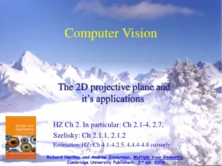
Computer Vision The 2D projective plane and it’s applications HZ Ch 2. In particular: Ch 2.1-4, 2.7, Szelisky: Ch 2.1.1, 2.1.2 Estimation:HZ: Ch 4.1-4.2.5, 4.4.4-4.8 cursorly Richard Hartley and Andrew Zisserman, Multiple View Geometry, Cambridge University Publishers, 2nd ed. 2004
Homogeneous coordinates Homogeneous coordinates but only 2DOF Inhomogeneous coordinates Homogeneous representation of 2D points and lines The point x lies on the line l if and only if Note that scale is unimportant for incidence relation equivalence class of vectors, any vector is representative Set of all equivalence classes in R3(0,0,0)T forms P2
The 2D projective plane X x X X Y y Y Y 0 Z Z l∞ Projective point X∞ Homogeneous coordinates s s 0 X 1 Inhomogeneous equivalent = Z Y • Perspective imaging models 2d projective space • Each 3D ray is a point in P2 : homogeneous coords. • Ideal points • P2 is R2 plus a “line at infinity” X∞ = l∞
Lines X Y Z X A 0 Y 0 B 0 1 C For any 2d projective property, a dual property holds when the role of points and lines are interchanged. Duality: l = X1 X2 l1 l2 X = • Projective line ~ a plane through the origin l = = X lTX = XTl = AX + BY + CZ = 0 X l∞ l = X∞ = “line at infinity” • Ideal line ~ the plane parallel to the image HZ The line joining two points The point joining two lines
Points from lines and vice-versa Line joining two points The line through two points and is Intersections of lines The intersection of two lines and is Example Note: with
Ideal points and the line at infinity tangent vector normal direction Example Ideal points Line at infinity Intersections of parallel lines Note that in P2 there is no distinction between ideal points and others
Conics or homogenized or in matrix form with Curve described by 2nd-degree equation in the plane 5DOF:
Five points define a conic stacking constraints yields For each point the conic passes through or
Tangent lines to conics The line l tangent to C at point x on C is given by l=Cx l x C
Dual conics In general (C full rank): A line tangent to the conic C satisfies Dual conics = line conics = conic envelopes
Degenerate conics Note that for degenerate conics A conic is degenerate if matrix C is not of full rank e.g. two lines (rank 2) e.g. repeated line (rank 1) Degenerate line conics: 2 points (rank 2), double point (rank1)
Conics • Conic: • Euclidean geometry: hyperbola, ellipse, parabola & degenerate • Projective geometry: equivalent under projective transform • Defined by 5 points • Tangent line • Dual conic C* inhomogeneous homogeneous
Projective transformations • Homographies, collineations, projectivities • 3x3 nonsingular H maps P2 to P2 8 degrees of freedom determined by 4 corresponding points • Transforming Lines? subspaces preserved substitution dual transformation
Planar Projective Warping HZ A novel view rendered via four points with known structure
Planar Projective Warping HZ Original Top-down Facing right Artifacts are apparent where planarity is violated...
2d Homographies 2 images of a plane 2 images from the same viewpoint (Perspectivity)
Panoramic imagingAppl: Quicktime VR, robot navigation etc. Homographies of the world, unite!
The line at infinity The line at infinity l is a fixed line under a projective transformation H if and only if H is an affinity Note: But points on l can be rearranged to new points on l
Affine properties from images Projection (Imaging) Rectification Post-processing
Affine rectification l∞ v1 v2 l1 l3 l2 l4 Point transformation for Aff Rect: Exercise: Verify
Geometric strata: 2d overview l ¥ C* C* ¥ ¥ 2 dof l ¥ 2 dof
Parameter estimation in geometric transforms cs499 Useful in Grad research • 2D homography Given a set of (xi,xi’), compute H (xi’=Hxi) • 3D to 2D camera projection Given a set of (Xi,xi), compute P (xi=PXi) • Fundamental matrix Given a set of (xi,xi’), compute F (xi’TFxi=0) • Trifocal tensor Given a set of (xi,xi’,xi”), compute T
Math tools 1:Solving Linear Systems • If m=n (A is a square matrix), then we can obtain the solution by simple inversion: • If m>n, then the system is over-constrained and Ais not invertible • Use Matlab “\” to obtain least-squares solutionx= A\b to Ax =b internally Matlab uses QR-factorization (cmput418/340) to solve this. • Can also write this using pseudoinverse A+ =(ATA)-1AT to obtain least-squares solutionx= A+b
Fitting Lines • A 2-D point x = (x, y) is on a line with slope m and intercept b if and only if y =mx + b • Equivalently, • So the line defined by two points x1, x2 is the solution to the following system of equations:
Fitting Lines • With more than two points, there is no guarantee that they will all be on the same line • Least-squares solution obtained from pseudoinverse is line that is “closest” to all of the points courtesy of Vanderbilt U.
Example: Fitting a Line • Suppose we have points (2, 1), (5, 2), (7, 3), and (8, 3) • Then and x = A+b =(0.3571, 0.2857)T Matlab: x = A\b
Homogeneous Systems of Equations • Suppose we want to solve Ax = 0 • There is a trivial solution x = 0, but we don’t want this. For what other values of x is Ax close to 0? • This is satisfied by computing the singular value decomposition (SVD) A = UDVT (a non-negative diagonal matrix between two orthogonal matrices) and taking x as the last column of V • Note that Matlab returns [U, D, V] = svd(A)
Line-Fitting as a Homogeneous System • A 2-D homogeneous point x = (x, y, 1)T is on the line l = (a, b, c)T only when ax + by + c = 0 • We can write this equation with a dot product: x•l = 0,and hence the following system is implied for multiple points x1, x2, ..., xn:
Example: Homogeneous Line-Fitting • Again we have 4 points, but now in homogeneous form: (2, 1, 1), (5, 2, 1), (7, 3, 1), and (8, 3, 1) • Our system is: • Taking the SVD of A, we get: compare tox =(0.3571, 0.2857)T
Parameter estimation in geometric transforms cs499 Useful in Grad research • 2D homography Given a set of (xi,xi’), compute H (xi’=Hxi) • 3D to 2D camera projection Given a set of (Xi,xi), compute P (xi=PXi) • Fundamental matrix Given a set of (xi,xi’), compute F (xi’TFxi=0) • Trifocal tensor Given a set of (xi,xi’,xi”), compute T
Estimating Homography Hgiven image points x HZ A novel view rendered via four points with known structure
Number of measurements required • At least as many independent equations as degrees of freedom required • Example: 2 independent equations / point 8 degrees of freedom 4x2≥8
Approximate solutions • Minimal solution 4 points yield an exact solution for H • More points • No exact solution, because measurements are inexact (“noise”) • Search for “best” according to some cost function • Algebraic or geometric/statistical cost
Many ways to solve: Different Cost functions => differencesin solution • Algebraic distance • Geometric distance • Reprojection error • Comparison • Geometric interpretation
Gold Standard algorithm • Cost function that is optimal for some assumptions • Computational algorithm that minimizes it is called “Gold Standard” algorithm • Other algorithms can then be compared to it
Estimating H: The Direct Linear Transformation (DLT) Algorithm • xi =HXiis an equation involving homogeneous vectors, so HXi and xi need only be in the same direction, not strictly equal • We can specify “same directionality” by using a cross product formulation:
Direct Linear Transformation(DLT) • Equations are linear in h • Only 2 out of 3 are linearly independent (indeed, 2 eq/pt) (only drop third row if wi’≠0) • Holds for any homogeneous representation, e.g. (xi’,yi’,1)
Direct Linear Transformation(DLT) • Solving for H size A is 8x9 or 12x9, but rank 8 Trivial solution is h=09T is not interesting 1-D null-space yields solution of interest pick for example the one with
Direct Linear Transformation(DLT) • Over-determined solution No exact solution because of inexact measurement i.e. “noise” • Find approximate solution • Additional constraint needed to avoid 0, e.g. • not possible, so minimize
DLT algorithm • Objective • Given n≥4 2D to 2D point correspondences {xi↔xi’}, determine the 2D homography matrix H such that xi’=Hxi • Algorithm • For each correspondence xi ↔xi’ compute Ai. Usually only two first rows needed. • Assemble n 2x9 matrices Ai into a single 2nx9 matrix A • Obtain SVD of A. Solution for h is last column of V • Determine H from h (reshape)
Inhomogeneous solution Since h can only be computed up to scale, pick hj=1, e.g. h9=1, and solve for 8-vector Solve using Gaussian elimination (4 points) or using linear least-squares (more than 4 points) However, if h9=0 this approach fails also poor results if h9 close to zero Therefore, not recommended for general homographies Note h9=H33=0 if origin is mapped to infinity
Normalizing transformations Or • Since DLT is not invariant to coordinate transforms, what is a good choice of coordinates? e.g. • Translate centroid to origin • Scale to a average distance to the origin • Independently on both images
Normalized DLT algorithm • Objective • Given n≥4 2D to 2D point correspondences {xi↔xi’}, determine the 2D homography matrix H such that xi’=Hxi • Algorithm • Normalize points • Apply DLT algorithm to • Denormalize solution
Importance of normalization 1 ~104 ~102 ~102 ~102 ~102 ~102 1 ~104 orders of magnitude difference!
Degenerate configurations Define: Then, x1 x1 x1 x4 x4 x4 x2 H? H’? x2 x2 x3 x3 x3 (case B) (case A) i=1,2,3,4 Constraints: H* is rank-1 matrix and thus not a homography If H* is unique solution, then no homography mapping xi→xi’(case B) If further solution H exist, then also αH*+βH (case A) (2-D null-space in stead of 1-D null-space)
First 3D proj geom • Then review and more on camera models • Then following P estimation
A 3D Vision Problem: Multi-view geometry - resection • Projection equation xi=PiX • Resection: • xi,X Pi Given image points and 3D points calculate camera projection matrix.

