Download
1 / 26
270 likes | 342 Vues
Explore the Jablonski Diagram and the life history of excited state electrons in luminescent probes. Learn about fluorescence, absorption, and deexcitation processes, as well as how to measure fluorescence lifetimes.

E N D
Fluorescence Lifetimes Martin Hof, Radek Macháň
The Jablonski Diagram The life history of an excited state electron in a luminescent probe Internal conversion ki ~ 1012 s-1 S2 Radiationlessdecayknd >1010 s-1 ki ~ 106 -1012 s-1 Inter-system crossing kx ~ 104 – 1012 s-1 S1 T1 kx ~ 10-1 – 105 s-1 Fluorescence kf ~ 107 – 109 s-1 Absorption Phosphorescence kph < 106 s-1 S0 • Fluorescence is observed if kf~>ki+kx • The time a molecule spends in the excited state is determined by the sum of the kinetic constants of all deexcitation processes
What is meant by the “lifetime” of a fluorophore??? Absorption and emission processes are almost always studied on populations of molecules and the properties of the supposed typical members of the population are deduced from the macroscopic properties of the process. In general, the behavior of an excited population of fluorophores is described by a familiar rate equation: k where n* is the number of excited elements at time t, k is the rate constant of all deexcitation processes and f(t) is an arbitrary function of the time, describing the time course of the excitation. The dimensions of k are s-1 (transitions per molecule per unit time).
If excitation is switched off at t = 0, the last equation, takes the form: k and describes the decrease in excited molecules at all further times. Integration gives: k The lifetimeis equal to k-1 If a population of fluorophores are excited, the lifetime is the time it takes for the number of excited molecules to decay to 1/e or 36.8% of the original population according to:
The deexcitation ratek is the sum of the rates of all possible deexcitation pathways: k = kf +ki + kx + kET + …= kf + knr kf is the rate of fluorescence, ki the rate of internal conversion and vibrational relaxation, kx the rate of intersystem crossing, kET the rate of inter-molecular energy transfer and knr is the sum of rates of radiationless deexcitation pathways. • non-radiative processes: • isolated molecules in “gas-phase” only internal conversion and intersystem crossing • in condensed phase additional pathways due to interaction with molecular environment: excited state reactions, energy transfer,…
ANS in water is ~100 picoseconds but can be 8 – 10 ns bound to proteins Ethidium bromide is 1.8 ns in water, 22 ns bound to DNA and 27ns bound to tRNA The lifetime of tryptophan in proteins ranges from ~0.1 ns up to ~8 ns • non-radiative processes: • isolated molecules in “gas-phase” only internal conversion and intersystem crossing • in condensed phase additional pathways due to interaction with molecular environment: excited state reactions, energy transfer,… Note: fluorescence lifetime tends to be shorter in more polar environment, because larger dipole moments of surrounding molecules can increase the efficiency of energy transfer
The radiation lifetimetr = kf-1 is practically a constant for a given molecule The fluorescence lifetime t= k-1 = (kf + knr)-1 depends on the environment of the molecule through knr. Fluorescence quantum yield: is proportional to fluorescence lifetime. Addition of another radiationless pathway increases knr and, thus, decreases t and QY. However, the measurement of fluorescence lifetime is more robust than measurement of fluorescence intensity (from which the QY is determined), because it depends on the intensity of excitation nor on the concentration of the fluorophores. The fluorescence intensityI (t) = kfn*(t) is proportional to n*(t) and vice versa
How to measure fluorescence lifetime ??? Time (or pulsed) domain Frequency (or harmonic) domain t Molecules are excited by a very short pulse (close to a d-pulse) at t = 0 and the decay of florescence intensity is measured. Usually by Time Correlated Single Photon Counting (TCSPC) Excitation light is harmonically modulated with circular frequency w and so is the emission. Fluorescence lifetime can be deduced from the phase shift f and modulation m.
Time (or pulsed) domain Ideal single-exponential decay of fluorescence intensity (excited by a d-pulse at t = 0) The realfluorescence decay is a convolution with the profile of the excitation pulse The measuredfluorescence decay is a convolution of the real decay with the response of the detection The instrument response functioniREF is typically measured as a response of the instrument to scattered excitation pulse. The parameters of I(t) (the lifetime t) are usually obtained by nonlinear fitting combined with a deconvolution procedure. The deconvolution is not necessary when the excitation pulse is very short compared to the lifetime (fs-lasers) and/or high precision of lifetime determination is not required. A part of the measured decay closest to the excitation pulse is then excluded from the analysis (“tail fitting”).
Time (or pulsed) domain multi-exponential decay (at least two distinct lifetimes) single-exponential decay An analogous analysis is performed in the case of multi-exponential decay to extract lifetimes ti and fractions ai. An increase in the number of fitted parameters represents increases the risk of artefacts (more than 3 lifetimes not recommended) Alternatively maximum entropy method can be used – allows analysis of continuous distributions of lifetimes. Mean lifetime – an average time a molecule spends in the excited state
Time correlated single photon counting (TCSPC) monochromator / filter pulsed laser sample trigger pulse from a reference detector and discriminator or from the pulse generator which drives the laser pulses monochromator / filter detector TAC discriminator START STOP multichannel analyzer generates an array of numbers of detected photons within short time intervals – photon arrival histogram detector: multichannel plate photomultiplier tube (MCP PMT), avalanche photo diode (APD)
Discriminator eliminates noise (dark counts of the photodetector) and generates pulses which are independent of the actual shape and amplitude of the detector pulse (which is generated when a photon hits the detector) • Leading edge discriminator • the pulse timing depends on its amplitude increases time jitter voltage threshold Dt time • Constant fraction discriminator • the signal is divided to two branches, the signal in one branch is inverted and in the other delayed and then they are added together • the zero point used for timing independent of amplitude (1-f) I(t-d) - fI(t)
Time to Amplitude Converter (TAC) 10 V • TAC generates a linear voltage ramp by charging a capacitor • TAC is the limiting step in TCSPC voltage • the charging is started by a trigger pulse (synchronized with the excitation pulse) START STOP 50 ps time • the charging is stopped by a pulse from the detector (photon arrival) and the reached voltage is stored by the multichannel analyzer. • if no photon is detected TAC is reset when reaching the maximum voltage • TACs are usually operated in reverse mode: • the charging is triggered by photon arrival and stopped by the excitation pulse • the capacitor is charged in those excitation cycles when a photon is detected
Time correlated single photon counting (TCSPC) monochromator / filter pulsed laser sample monochromator / filter reference pulse voltage detector TAC time to amplitude convertor discriminator STOP START value of voltage reached multichannel analyzer generates an array of numbers of detected photons within short time intervals – photon arrival histogram
TCSPC - Artefacts If more photons arrive within a single time interval (ti + Dt) after excitation, only a single count is registered – the discriminator does not take into account the size of the pulse from the detector once it is larger than the discrimination level The average number of photonswi reaching the detector with each interval (ti + Dt) should be less then one Dt TAC however detects only one photon in each excitation cycle The average number of photons reaching the detector in each excitation cycle should be less then one
TCSPC - Theory Consider thatwithin one excitation cycle in the time interval (ti + Dt) after excitation (which corresponds to the i-th channel of the multichannel analyzer) on average wi photons reach the detector. The probability of z photons reaching the detector in that interval is given by Poisson distribution: Specifically: After many (NE) excitation cycles, Ni counts will be detected in the i-th interval Low intensities are used in TCSPC, therefore wi << 1 and: The number of counts in the i-th interval is indeed proportional to the intensity in the interval (ti + Dt).
TCSPC - Theory TAC however detects only one photon in each excitation cycle The actual number of counts NSi stored in the i-th channel of the multichannel analyzer is lower than Ni. That is called the pile-up effect To prevent the need for corrections of the measured decays for pile-up effect very low intensities are used to make the effect negligible. The intensities are usually adjusted to ensure that Niis approximately1%ofNE, that means that a photon is detected only in 1% of excitation cycles. High repetition rates of excitation pulses are used to decrease the time necessary for measurement. However, the fluorescence intensity has to decay completely between the pulses – repetition rates usually ≈ 1 – 10 MHz. Note: an advantage of TCSPC is the known statisticaldistribution ofnoise (Poisson distribution) and it can be included in the data analysis.
Here are pulse decay data on anthracene in cyclohexane taken on an IBH 5000U Time-correlated single photon countinginstrument equipped with a LED short pulse diode excitation source. t = 4.1nsc2 = 1.023 56ps/ch
Time domain – An alternative detection method The decay of fluorescence can be also recorded with high temporal resolution using a streak camera (analogous to an oscilloscope) voltage sweep phosphor screen photon photoelectron photocathode Modern streak cameras have time resolution superior to photomulpliers. Parallel detection in all channels – intensity is not limited by pile-up effect.
Frequency (harmonic) domain The frequency domain measurement does not provide a direct information on the shape of the fluorescence decay The equality of tfand tm indicates single-exponential decay. If they are not equal, more general expressions have to be used. High excitation intensity can be applied to shorten the measurement time
Frequency (harmonic) domain - derivation derivation of equations for a single-exponential decay: considering the harmonic excitation: we assume a solution in the form: to ensure that the equation is solved for all values of t, we search for such values of phase shift f and modulation m that satisfy the equality of terms containing t, terms containing cos(wt) and terms containing sin(wt) on both sides of the equation.
Frequency (harmonic) domain – general expressions An integral transform of the fluorescence decayI(t) gives: The excitation intensity is harmonically modulated by a Pockels cell or a harmonically modulated LED or laser diode is used. The frequency is typically in the range of ~10 – 100 MHz
An example of the use of lifetime data is given by a study of a rhodamine labeled peptide which can be cleaved by a protease (from Blackman et al. (2002) Biochemistry 41:12244) Weak fluorescence E1 Strong fluorescence N D N I D A A I D S S D I V I V C C C C R h o R h o R h o In the intact peptide the rhodamine molecules form a ground-state dimer with a low quantum yield (green curve). Upon cleavage of the peptide the rhodamine dimer breaks apart and the fluorescence is greatly enhanced (blue curve). Lifetime data allow us to better understand the photophysics of this system
Weak fluorescence E1 Strong fluorescence N D N I D A A I D S S D I V I V C C C C R h o R h o R h o Lifetime data for two rhodamine isomers (5’ and 6’) linked to the peptide As the lifetime data indicate, before protease treatment the rhodamine lifetime was biexponential with 95% of the intensity due to a long component and 5% due to a short component. Hence one can argue that the intact peptide exists in an equilibrium between open (unquenched) and closed (quenched) forms.
E2 Hydrophobicity – sensing with lifetime sensitive dyes exc = 467 nm 100×, 1.3 N.A. oil immersion 300 × 300 pixels acquisition time: 2 ms/pixel fluorescence lifetime image of a part of a membrane of a living hepatocyte cell stained with the dye NBD (7-nitrobenz-2-oxa-1,3-diazole) → lifetime is depending on the hydrophobicity of the environment Fluorescence intensity Fluorescence lifetime Lifetime distribution