Lecture 3: Simple Keynesian Model

Lecture 3:Simple Keynesian Model National Income Determination Three-Sector National Income Model

Outline • Three-Sector Model • Output-Expenditure Approach: Equilibrium National Income Ye • Injection-Withdrawal Approach: Equilibrium National Income Ye • Fiscal Policy

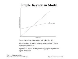
Three-Sector Model • With the introduction of the government sector (i.e. together with households C, firms I), aggregate expenditure E consists of one more component, government expenditure G. E = C + I + G • Still, the equilibrium condition is Planned Y = Planned E

Three-Sector Model • Government expenditure is made up of two parts • Government expenditure on current production, G • Transfer payments, Q • Government also collects tax revenues, T • Government budget may be defined as • T- (G + Q) • When positive, there is a government surplus • When negative, there is a government deficit • When zero, there is a balanced budget

Three Sector Model • Assumptions about the Government component of AE • Government expenditure on current production is assumed constant, G= G* • Transfer payments are also an autonomous expenditure flow, Q= Q* • Additional assumptions • All transfer payments are made to households • All taxes are direct taxes on personal and company incomes • Tax rate is levied at a flat rate, T= tY where 0<t<1 • i.e. taxes are a constant proportion of national income

Three-Sector model • In the 2-sector model, all national income was paid out to households • Households decided to consume or save amounts • National income, Y= disposable income, Yd • Introduction of taxes and transfer payments drives a wedge between national income and disposable income • Yd= Y- T + Q

Three- Sector Model • We continue to assume C= cYd • Households spend a fraction of disposable income and save the rest • Given that Yd= Y-T+Q, • C= c(Y-T+Q) =cY – cT + cQ, but T= tY =cY – ctY + cQ = c(1 – t) Y + cQ

The Income-Expenditure Approach • Aggregate expenditure has three components • E= C + I + G • At the equilibrium, • E = Y • Derive the aggregate expenditure function assuming the following • Yd = Y – T + Q • G= G* • Q= Q* • T= tY • I= I* • C= cYd

The Income-Expenditure Approach • E= C + I + G = cYd + I* + G* = c( Y – T+ Q*) + I* + G* = c(Y – tY + Q*) + I* + G* At equilibrium, Y= E Y = c(1-t) Y+ cQ* + I* + G* Y- c(1 – t) Y= cQ* + I* + G* Y[1 – c(1 – t)] = cQ* + I* + G* Y = 1/ [1 – c(1 – t)] (cQ* + I* + G*) • Expenditure depends on two main terms • The sum of the three autonomous flows: Q*, I*, G* • Behavioural patterns of consumption, c, and taxation, t

Changes in Equilibrium Income • What is the effect of changes in autonomous expenditure flows and the tax rate, t, on national income?

A change in G* and/or I* • An increase in G or I shifts the AE curve upwards • Increase in national income

A change in transfer payments • An increase in transfer payments will also increase national income • How? • However, an extra Ghc1 spent on final government expenditure, G, increases national income by more than Ghc1 spent on transfer payment, Q. • Why?

A change in tax rate • A cut in tax rates implies that a larger proportion of each Ghc1 reaches households as disposable income • Therefore, the propensity to consume increases • AE becomes steeper • Increase in national income

The Multiplier • How large is the change in national income from a given change in autonomous expenditure? • To determine this, we need to solve the following algebraically: • Ye/I • Ye/G • Ye/Q

The Multiplier • Recall from the income expenditure approach • Equilibrium national income is given by Y = 1/ [1 – c(1 – t)] (cQ* + I* + G*) • Solution? • Ye/I • Ye/G • Ye/Q • What do you notice about the change in income from a change in investment, I*, or government expenditure, G*? • What do you notice about the value of the transfer payments multiplier, Q*? • Is it larger or smaller? Why? • Under what conditions are al three multipliers equal?

Injection-Withdrawal Approach • In a 3-sector model, national income is either consumed, saved or taxed by the government • Y = C + S + T • Given E = C + I + G • In equilibrium, Y = E • C + S + T = C + I + G •  S + T = I + G , but G= G + Q (Q= cQ) •  S + T = I + G + cQ i.e. withdrawals = injections

Injections- Withdrawals Approach:Equilibrium national income • Graphical Approach

Injections- Withdrawals Approach:Equilibrium national income • Graphical Approach • An increase in any component of aggregate expenditure shifts the injections curve upwards • And vice versa • A fall in the tax rate increases the amount of disposable income, and the propensity for increased consumption • This is illustrated by a flatter (i.e. smaller value of t) withdrawals curve, leading to increased equilibrium national income

Injections- Withdrawals Approach:Equilibrium national income • An algebraic approach • We define savings, S= s(Y- T) • i.e. the part of national income that is saved • Other assumptions • T= tY • Q= Q* • I= I* • G= G* • At the equilibrium, Withdrawals = Injections • Withdrawals = s(1- t)Y + tY = Y[s(1- t) + t] • Injections = I* + G* + cQ* • At the equilibrium, • Y =1/ [s(1- t) + t] x (I* + G* + cQ*) • Is this the same equilibrium as obtained under the income-expenditure approach? • Derive the multipliers for investment and government expenditures, and transfer payments.

Limitation of the Simple Keynesian model • Y = Multiplier* G* • There are several problems with this method of analysis, i.e., Y may be less • Sources of financing G* • Effects on private investment I* • Productivity of government projects

The Problems of the Simple Keynesian Multiplier k E • Sources of financing G’ • Increasing Tax • will exert a contractionary effect on the economy • Increasing Money Supply • will generate an inflationary pressure • Prices assumed constant • Increasing Debt/ Private sector borrowing • will increase the demand for loanable fund as well as interest rate  affect private investment

The Problems of the Simple Keynesian Multiplier k E • Effects on Private Investment I’ • Private investment may be crowded out when government increases its expenditure • It is questionable that the government can really produce something which is desired by the consumers • Besides, government investment projects are usually less productive than private investment projects

The Problems of the Simple Keynesian Multiplier k E • Productivity of Government Projects • Government projects may not yield a rate of return (MEC / MEI) exceeding the market interest rate.

Take- Home Assignment • Using the mechanistic Keynes Theory of National Income, explain the causes and solutions to the Great Depression of 1929.

Next Class • Money and its Functions • The origin of money • Modern money and definition of monetary aggregates • Commercial Banks and Money Creation • The Central Bank and its functions

Lecture 3: Simple Keynesian Model