Text Exercise 1.38 (a) (b)

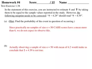
1. Homework #4 Score____________ / 15 Name ______________ Text Exercise 1.38 (a) (b) In the statement of this exercise, you are instructed to estimate  and  by taking them to be equal to the sample values reported in the study. However, the following misprint needs to be corrected: “ = 4.29” should read “ = 4.59”. (Hint: Find the probability of the event in question of occurring.) Since practically no samples of size n = 50 CAHS scores have a mean more than 6, we do not expect to observe this. Actually observing a sample of size n = 50 with mean of 6.2 would make us conclude that  = 4.59 is not true.

2. Text Exercise 1.42 (a) (b) (c) (No matter what method you use to do the necessary calculations, you should be able to verify that y = 1.073 and s = 0.2316.)  — = 2 0.025  — = 2 0.025 6 n = y = s = 1.073 0.2316 1 –  = 0.95 df = t0.025 = 5 2.571 1.073 – (2.571)(0.2316/6) , 1.073 + (2.571)(0.2316/6) 0.830 , 1.316 We can be 95% confident that the mean decay rate of fine particles produced from oven cooking or toasting is between 0.830 and 1.316 m/hour, Among all possible samples of size n = 6, 95% of these samples yield a confidence interval that actually contains the population mean. Either the population of decay rates has a normal distribution the sample size n = 6 is sufficiently large so that y has a normal (or approximate) distribution.

3. Text Exercise 1.46 (a) (b) Text Exercise 1.48 Answer this question by considering a hypothesis test H0:  = 8 vs. H1:   8 where the t test statistic is used. Indicate whether or not each of the following changes could affect the rejection region for this hypothesis test: The hypothesized mean value 8 is changed to 20. The sample size n is changed. The significance level  is changed. The alternative hypothesis is changed to H1:  > 8 . The rejection region remains the same. The rejection region could change. The rejection region could change. The rejection region could change. Rejecting H0 provides strong evidence to support H1 but does not prove H1 is true. Write each hypothesis first in words, then using the appropriate symbol(s). H0: H1: The mean listening time is equal to 9 seconds, that is,  = 9. The mean listening time is different from 9 seconds, that is,  9.

4. Additional HW Exercise #1.9 - continued Step 15: The output title Means can be deleted. Use the File> Print options to obtain a printed copy of the sample statistics. Since there is no need for you to save the output, you may close the SPSS output window without saving the results, after you have your printed copy of the output. Attach this printed copy to this assignment before submission. Exit from SPSS. (b) Find and interpret a 95% confidence interval for the mean yearly income ($1000s) of voters in the state.  — = 2 0.025  — = 2 0.025 30 n = y = s = 45.40 15.895 1 –  = 0.95 These statistics are on the SPSS output. df = t0.025 = 29 2.045 45.40 – (2.045)(15.895/30) , 45.40 + (2.045)(15.895/30) 39.465 , 51.335 We can be 95% confident that the mean yearly income of voters in the state is between 39.465 and 51.335 thousand dollars,