Sample Geometry and Random Sampling
Sample Geometry and Random Sampling. Shyh-Kang Jeng Department of Electrical Engineering/ Graduate Institute of Communication/ Graduate Institute of Networking and Multimedia. Array of Data. * a sample of size n from a p -variate population. Row-Vector View. Example 3.1.

Sample Geometry and Random Sampling
E N D
Presentation Transcript
Sample Geometry and Random Sampling Shyh-Kang Jeng Department of Electrical Engineering/ Graduate Institute of Communication/ Graduate Institute of Networking and Multimedia
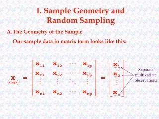
Array of Data *a sample of size n from a p-variate population
Random Sample • Row vectors X1’, X2’, …, Xn’ represent independent observations from a common joint distribution with density function f(x)=f(x1, x2, …, xp) • Mathematically, the joint density function of X1’, X2’, …, Xn’ is
Random Sample • Measurements of a single trial, such as Xj’=[Xj1,Xj2,…,Xjp], will usually be correlated • The measurements from different trials must be independent • The independence of measurements from trial to trial may not hold when the variables are likely to drift over time
Geometric Interpretation of Randomness • Column vector Yk’=[X1k,X2k,…,Xnk] regarded as a point in n dimensions • The location is determined by the joint probability distribution f(yk) = f(x1k, x2k,…,xnk) • For a random sample, f(yk)=fk(x1k)fk(x2k)…fk(xnk) • Each coordinate xjk contributes equally to the location through the same marginal distribution fk(xjk)
Interpretation in p-space Scatter Plot • Equation for points within a constant distance c from the sample mean
Result 3.2 • The generalized variance is zero when the columns of the following matrix are linear dependent
Examples Cause Zero Generalized Variance • Example 1 • Data are test scores • Included variables that are sum of others • e.g., algebra score and geometry score were combined to total math score • e.g., class midterm and final exam scores summed to give total points • Example 2 • Total weight of chemicals was included along with that of each component
Result 3.3 • If the sample size is less than or equal to the number of variables ( ) then |S| = 0 for all samples
Result 3.4 • Let the p by 1 vectors x1, x2, …, xn, where xj’ is the jth row of the data matrix X, be realizations of the independent random vectors X1, X2, …, Xn. • If the linear combination a’Xj has positive variance for each non-zero constant vector a, then, provided that p < n, S has full rank with probability 1 and |S| > 0 • If, with probability 1, a’Xj is a constant c for all j, then |S| = 0
Volume Generated by Deviation Vectors of Standardized Variables