Analysis of Variance
Analysis of Variance. Chapter 13 BA 303. An Introduction to Analysis of Variance. A factor is a variable that the experimenter has selected for investigation. A treatment is a level of a factor. Example:

Analysis of Variance
E N D
Presentation Transcript
Analysis of Variance Chapter 13 BA 303
An Introduction to Analysis of Variance • A factor is a variable that the experimenter has selected for investigation. • A treatment is a level of a factor. • Example: • A company president is interested in the number of hours worked by managers at three different plants: Gulfport, Long Beach, and Biloxi. • Factor: Plant • Treatment: Gulfport, Long Beach, and Biloxi
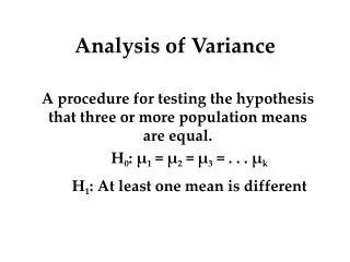
Analysis of Variance: A Conceptual Overview Analysis of Variance (ANOVA) can be used to test for the equality of three or more population means. Data obtained from observational or experimental studies can be used for the analysis. We want to use the sample results to test the following hypotheses: H0: 1=2=3=. . . = k Ha: Not all population means are equal
Analysis of Variance: A Conceptual Overview H0: 1=2=3=. . . = k Ha: Not all population means are equal If H0 is rejected, we cannot conclude that all population means are different. Rejecting H0 means that at least two population means have different values.
Analysis of Variance: A Conceptual Overview • Assumptions for Analysis of Variance For each population, the response (dependent) variable is normally distributed. The variance of the response variable, denoted 2, is the same for all of the populations. The observations must be independent.
Sampling Distribution of Given H0 is True Analysis of Variance: A Conceptual Overview Sample means are close together because there is only one sampling distribution when H0 is true.
Sampling Distribution of Given H0 is False Analysis of Variance: A Conceptual Overview 3 1 2 Sample means come from different sampling distributions and are not as close together when H0 is false.
Analysis of Variance • Between-Treatments Estimate of Population Variance • Within-Treatments Estimate of Population Variance • Comparing the Variance Estimates: The F Test • ANOVA Table
Between-Treatments Estimate of Population Variance s 2 • The estimate of 2 based on the variation of the sample means is called the mean square due to treatmentsand is denoted by MSTR. Numerator is called the sum of squares due to treatments(SSTR) Denominator is the degrees of freedom associated with SSTR
Within-Treatments Estimateof Population Variance s 2 • The estimate of 2 based on the variation of the sample observations within each sample is called the mean square error and is denoted by MSE. Numerator is called the sum of squares due to error(SSE) Denominator is the degrees of freedom associated with SSE
Comparing the Variance Estimates: The F Test • If the null hypothesis is true and the ANOVA • assumptions are valid, the sampling distribution of • MSTR/MSE is an F distribution with MSTR d.f. • equal to k - 1 and MSE d.f. equal to nT - k. • If the means of the k populations are not equal, the • value of MSTR/MSE will be inflated because MSTR • overestimates 2. • Hence, we will reject H0 if the resulting value of • MSTR/MSE appears to be too large to have been • selected at random from the appropriate F • distribution.
Comparing the Variance Estimates: The F Test • Sampling Distribution of MSTR/MSE Sampling Distribution of MSTR/MSE Reject H0 a Do Not Reject H0 MSTR/MSE F Critical Value
ANOVA Table for a Completely Randomized Design p- Value Source of Variation Sum of Squares Degrees of Freedom Mean Square F Treatments k - 1 SSTR Error SSE nT - k Total SST nT - 1 SST’s degrees of freedom (d.f.) are partitioned into SSTR’s d.f. and SSE’s d.f. SST is partitioned into SSTR and SSE.
ANOVA Table for a Completely Randomized Design SST divided by its degrees of freedom nT – 1 is the overall sample variance that would be obtained if we treated the entire set of observations as one data set. With the entire data set as one sample, the formula for computing the total sum of squares, SST, is:
ANOVA Table for a Completely Randomized Design ANOVA can be viewed as the process of partitioning the total sum of squares and the degrees of freedom into their corresponding sources: treatments and error. Dividing the sum of squares by the appropriate degrees of freedom provides the variance estimates and the F value used to test the hypothesis of equal population means.
Test for the Equality of k Population Means • Hypotheses H0: 1=2=3=. . . = k Ha: Not all population means are equal • Test Statistic F = MSTR/MSE
Test for the Equality of k Population Means • Rejection Rule Reject H0 if p-value <a p-value Approach: Critical Value Approach: Reject H0 if F>Fa where the value of F is based on an F distribution with k - 1 numerator d.f. and nT - k denominator d.f.
Testing for the Equality of k Population Means Reed Manufacturing Janet Reed would like to know if there is any significant difference in the mean number of hours worked per week for the department managers at her three manufacturing plants (in Buffalo, Pittsburgh, and Detroit). An F test will be conducted using a = .05.
Testing for the Equality of k Population Means Reed Manufacturing A simple random sample of five managers from each of the three plants was taken and the number of hours worked by each manager in the previous week is shown on the next slide. Factor . . . Manufacturing plant Treatments . . . Buffalo, Pittsburgh, Detroit Experimental units . . . Managers Response variable . . . Number of hours worked
Testing for the Equality of k Population Means Plant 3 Detroit Plant 2 Pittsburgh Plant 1 Buffalo Observation 1 2 3 4 5 48 54 57 54 62 51 63 61 54 56 73 63 66 64 74 Sample Mean 55 68 57 Sample Variance 26.0 26.5 24.5
Testing for the Equality of k Population Means • p -Value and Critical Value Approaches 1. Develop the hypotheses. H0: 1= 2= 3 Ha: Not all the means are equal where: 1 = mean number of hours worked per week by the managers at Plant 1 2 = mean number of hours worked per week by the managers at Plant 2 3 = mean number of hours worked per week by the managers at Plant 3
= (55 + 68 + 57)/3 = 60 Testing for the Equality of k Population Means • p -Value and Critical Value Approaches a = .05 2. Specify the level of significance. 3. Compute the value of the test statistic. Mean Square Due to Treatments (Sample sizes are all equal.) SSTR = 5(55 - 60)2 + 5(68 - 60)2 + 5(57 - 60)2 = 490 MSTR = 490/(3 - 1) = 245
Testing for the Equality of k Population Means • p -Value and Critical Value Approaches 3. Compute the value of the test statistic. (con’t.) Mean Square Due to Error SSE = 4(26.0) + 4(26.5) + 4(24.5) = 308 MSE = 308/(15 - 3) = 25.667 F = MSTR/MSE = 245/25.667 = 9.55
Testing for the Equality of k Population Means • ANOVA Table Source of Variation Sum of Squares Mean Square Degrees of Freedom F p-Value 245 25.667 9.55 .0033 490 308 798 2 12 14 Treatment Error Total
Testing for the Equality of k Population Means • p –Value Approach 4. Compute the p –value. With 2 numerator d.f. and 12 denominator d.f., the p-value is .01 for F = 6.93. Therefore, the p-value is less than .01 for F = 9.55. 5. Determine whether to reject H0. The p-value < .05,so we reject H0. We have sufficient evidence to conclude that the mean number of hours worked per week by department managers is not the same at all 3 plant.
Testing for the Equality of k Population Means • Critical Value Approach 4. Determine the critical value and rejection rule. Based on an F distribution with 2 numerator d.f. and 12 denominator d.f., F.05 = 3.89. Reject H0 if F> 3.89 5. Determine whether to reject H0. Because F = 9.55 > 3.89, we reject H0. We have sufficient evidence to conclude that the mean number of hours worked per week by department managers is not the same at all 3 plant.
Perform an ANOVA Using the data in the table on the next slide, compute the mean and standard deviation for the Direct treatment. Compute the sum of the squares due to treatments (SSTR) and the mean square due to treatments (MSTR). Compute the sum of the squares due to the error (SSE) and the mean square due to the error (MSE). Compute the F test statistic. Using a=0.05, what do you conclude about the null hypothesis that the means of the treatments are equal? Determine the approximate p-value. Present the results in an ANOVA table.

