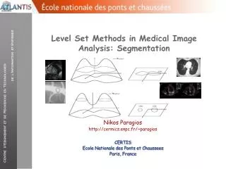
Level Set Methods in Medical Image Analysis: Segmentation
960 likes | 1.31k Vues
Level Set Methods in Medical Image Analysis: Segmentation. Nikos Paragios http://cermics.enpc.fr/~paragios CERTIS Ecole Nationale des Ponts et Chaussees Paris, France. Http://cermics.enpc.fr/~paragios/book/book.html. Nikos Paragios http://cermics.enpc.fr/~paragios Atlantis Research Group

Level Set Methods in Medical Image Analysis: Segmentation
E N D
Presentation Transcript
Level Set Methods in Medical Image Analysis: Segmentation Nikos Paragios http://cermics.enpc.fr/~paragios CERTIS Ecole Nationale des Ponts et Chaussees Paris, France
Http://cermics.enpc.fr/~paragios/book/book.html Nikos Paragios http://cermics.enpc.fr/~paragios Atlantis Research Group Ecole Nationale des Ponts et Chaussees Paris, France Stanley Osher http://math.ucla.edu/~sjo Department of Mathematics University of California, Los Angeles USA
Outline • Introduction/Motivation • On the Propagation of Curves • The snake model • The level set method • Basic Derivation, algorithms • Boundary-driven and Region-driven model free segmentation • The Level Set Method as a Direct Optimization Space • Multiphase Motion • Region-driven model free image segmentation • Knowledge-based Object Extraction • Shape Registration • Discussion
Motivation • Image Segmentation and image registration are core components of medical imaging • 2002 • The word “Segmentation” appears 34 times at MICCAI’02 program • The word “Registration” appears 22 times at MICCAI’02 program • 2003: • The word “Segmentation” appears 47 times at MICCAI’03 program ~ 25% • The word “Registration” appears 53 times at MICCAI’03 program ~ 25% • 2004: • The word “Segmentation” appears 51 times at MICCAI’04 program ~ 25% • The word “Registration” appears 67 times at MICCAI’04 program ~ 35%
Overview of Segmentation Techniques • Boundary-driven • Edge Detectors (model free) • Active Contours/snakes (model free + knowledge-based) • Active Shape Models (knowledge-based) • Region-driven • Deformable templates (knowledge-based) • Statistical/clustering techniques (model free + knowledge-based) • MRF-based techniques (model free) • Active Appearance Models (knowledge-based) • Boundary + Region-driven • Active Contours (model free + knowledge-based) • Graph-based Techniques (model free) • Level Set Methods (model free + knowledge-based)
On the Propagation of Curves • Snake Model (1987) [Kass-Witkin-Terzopoulos] • Planar parameterized curve C:R-->RxR • A cost function defined along that curve • The internal term stands for regularity/smoothness along the curve and has two components (resisting to stretching and bending) • The image term guides the active contour towards the desired image properties (strong gradients) • The external term can be used to account for user-defined constraints, or prior knowledge on the structure to be recovered • The lowest potential of such a cost function refers to an equilibrium of these terms
Active Contour Components • The internal term… • The first order derivative makes the snake behave as a membrane • The second order derivative makes the snake act like a thin plate • The image term… • Can guide the snake to • Iso-photes , edges • and terminations • Numerous Provisions…: balloon models, region-snakes, etc…
Optimizing Active Contours • Taking the Euler-Lagrange equations: • That are used to update the position of an initial curve towards the desired image properties • Initial the curve, using a certain number of control points as well as a set of basic functions, • Update the positions of the control points by solving the above equation • Re-parameterize the evolving contour, and continue the process until convergence of the process…
Pros/Cons of such an approach • Pros • Low complexity • Easy to introduce prior knowledge • Can account for open as well as closed structures • A well established technique, numerous publications it works • User Interactivity • Demetri Terzopoulos is a very good friend • Cons • Selection on the parameter space and the sampling rule affects the final segmentation result • Estimation of the internal geometric properties of the curve in particular higher order derivatives • Quite sensitive to the initial conditions, • Changes of topology (some efforts were done to address the problem)
The Level Set Method • Osher-Sethian (1987) • Earlier: Dervieux, Thomassett, (1979, 1980) • Introduced in the area of fluid dynamics • Vision and image segmentation • Caselles-Catte-coll-Dibos (1992) • Malladi-Sethian-Vermuri (1994) • Level Set Milestones • Faugeras-keriven (1998) stereo reconstruction • Paragios-Deriche (1998), active regions and grouping • Chan-Vese (1999) mumford-shah variant • Leventon-Grimson-Faugeras-etal (2000) shape priors • Zhao-Fedkiew-Osher (2001) computer graphics
The Level Set Method • Let us consider in the most general case the following form of curve propagation: • Addressing the problem in a higher dimension… • The level set method represents the curve in the form of an implicit surface: • That is derived from the initial contour according to the following condition:
The Level Set Method • Construction of the implicit function • And taking the derivative with respect to time (using the chain rule) • And we are DONE… (1)
The Level Set Method • Let us consider the arc-length (c) parameterization of the curve, then taking the directional derivative of in that dire- ction we will observe no change: • leading to the conclusion that the is ortho-normal to C where the following expression for the normal vector • Embedding the expression of the normal vector to: • the following flow for the implicit function is recovered: (2)
Level Set Method (the basic derivation) • Where a connection between the curve propagation flow and the flow deforming the implicit function was established • Given an initial contour, an implicit function is defined and deformed at each pixel according to the equation (2) where the zero-level set corresponds to the actual position of the curve at a given frame • Euclidean distance transforms are used in most of the cases as embedding function
Overview of the Method • The level set flow can be re-written in the following form • where H is known to be the Hamiltonian. Numerical approximations is then done according to the form of the Hamiltonian • Determine the initial implicit function (distance transform) • Evolve it locally according to the level set flow • Recover the zero-level set iso-surface (curve position) • Re-initialize the implicit function and Go to step (1) of the loop • Computationally expensive • Open Questions: re-initialization…and numerical approximations
Level Set Method and Internal Curve Properties • The normal to the curve/surface can be determined directly from the level set function: • The curvature can also be recovered from the implicit function, by taking the second order derivative at the arc length • Where we observe no variation since the implicit function has constant “zero” values, and given that as well as one can easily prove that: • That can also be extended to higher dimensions
Examples: Mean/Gaussian Curvature Flow • Minimize the Euclidean length of a curve/surface: • The corresponding level set variant with a distance transform as an implicit function: • Things become little bit more complicated at 3D (Gaussian Curvature) • Results are courtesy Prof. J. Sethian (Berkeley) & G. Hermosillo (INRIA)
From theory to Practice (Narrow Band) [Chop:93, Adalsteinsson-Sethian:95] • Central idea: we are interested on the motion of the zero-level set and not for the motion of each iso-phote of the surface • Extract the latest position • Define a band within a certain distance • Update the level set function • Check new position with respect the limits of the band • Update the position of the band regularly, and re-initialize the implicit function • Significant decrease on the computational complexity, in particular when implemented efficiently and can account for any type of motion flows
Narrow Band (the basic derivation) Results are courtesy: R. Deriche
Handling the Distance Function • The distance function has to be frequently re-initialized… • Extraction of the curve position & re-initialization: • Using the marching cubes one can recover the current position of the curve, set it to zero and then re-initialize the implicit function: the Borgefors approach, the Fast Marching method, explicit estimation of the distance for all image pixels… • Preserving the curve position and refinement of the existing function (Susman-smereka-osher:94) • Modification on the level set flow such that the distance transform property is preserved (gomes-faugeras:00) • Extend the speed of the zero level set to all iso-photes, rather complicated approach with limited added value?
From theory to Practice (Fast Marching)[Tsitsiklis:93,Sethian:95] • Central idea: “move” the curve one pixel in a progressive manner according to the speed function while preserving the nature of the implicit function • Consider the stationary equation • Such an equation can be recovered for all flows where the speed function has one sign (either positive or negative), propagation takes place at one direction • If T(x,y) is the time when the implicit function reaches (x,y):
Fast Marching (continued) • Consider the stationary equation in its discrete form: • And using the assumption that the surface propaga- tes in one direction, the so- lution can be obtained by outwards propagation from the smallest T value… • active pixels, the curve has already reached them • alive pixels, the curve could reach them at the next stage • far away pixels, the curve cannot reach them at this stage
Fast Marching (continued) • INITIAL STEP • Initialize for the all pixels of the front (active), their first order neighbors alive and the rest far away • For the first order neighbors, estimate the arrival time according to: • While for the rest the crossing time is set to infinity • PROPAGATION STEP • Select the pixel with the lowest arrival time from the alive ones • Change his label from alive to active and for his first order neighbors: • If they are alive, update their T value according to • If they are far away, estimate the arrival time according to:
Fast Marching Pros/Cons, Some Results • Fast approach for a level set implementation • Very efficient technique for re-setting the embedding function to be distance transform • Single directional flows, great importance on initial placement of the contours • Absence of curvature related terms or terms that depend on the geometric properties of the curve… • Results are courtesy: J. Sethian, R. Malladi, T. Deschamps, L. Cohen
Emigration from Fluid Dynamics to Vision • (Caselles-Cate-Coll-Dibos:93,Malladi-Sethian-Vemuri:94) have proposed geometric flows to boundary extraction • Where g(;) is a function that accounts for strong image gradients • And the other terms are application specific…that either expand or shrink constantly the initial curve • Distance transforms have been used as embedding functions Malladi-Sethian-Vemuri:94
Geodesic Active Contours[Caselles-Kimmel-Sapiro:95, Kichenassamy-Kumar-etal95] • Connection between level set methods and snake driven optimization • The geodesic active contour consists of a simplified snake model without second order smoothness • That can be written in a more general form as • Where the image metric has been replaced with a monotonically decreasing function:
Geodesic Active Contours[Caselles-Kimmel-Sapiro:95, Kichenassamy-Kumar-etal95] • Leading to the following more general framework… , • One can assume that smoothness as well as image terms are equally important and with some “basic math” • That seeks a minimal length geodesic curve attracted by the desired image properties…
Geodesic Active Contours • That when minimized leads to the following geometric flow: • Data-driven constrained by the curvature force • Gradient driven term that adjusts the position of the contour when close to the real 0bject boundaries… • By embedding this flow to a level set framework and using a distance transform as implicit function,
Geodesic Active Contours… • That has an extra term when compared with the flow proposed by Malladi-Sethian-Vemuri. • Single directional flow…requires the initial contour to either enclose the object or to be completely inside... Results are courtesy: R. Deriche
Gradient Vector Flow Geometric Contours[paragios-mellina-ramesh:01] • Initial conditions are an issue at the active contours since they are propagated mainly at one direction • Region terms (later introduced) is a mean to overcome this limitation… • an alternative is somehow to extend the boundary-driven speed function to account for directionality, thus recovering a field (u,v) • One can estimate this field close to the object boundaries…where • The image gradient at the boundaries is tangent to the curve • While the inward normal normal points towards the object boundaries
Gradient Vector Flow Geometric Contours[paragios-mellina-ramesh:01] • Let (f) be a continuous edge detector with values close to 1 at the presence of noise and 0 elsewhere… • The flow can be determined in areas with important boundary information (Important f) • And areas where there changes on f, |Gradient(f)| • While elsewhere recovering such a field is not possible and the only way to be done is through diffusion • This can be done through an approximation of image gradient at the edges and diffusion of this information for the rest of the image plane
Gradient Vector Flow Geometric Contours • This flow can be used within a geometric flow towards image segmentation… • The direction of the propagation should be the same with the one proposed by the recovered flow, therefore one can penalize the orientation between these two vectors. • That is integrated within the classical Geodesic active contour equation and is implemented using the level set function using the Additive Operator Splitting • The inner product between the curve normal and the vector field guides the curve propagation
Additive Operator Splitting[Weickert:98, Goldenberg-Kimmel:01] • Introduced for fast non-linear diffusion • Applied to the flow of the geodesic active contour • Where one can consider a signed Euclidean distance function to be the implicit function, leading to: • That can be written as: • That can be solved in an explicit form: • Or a semi-implicit one:
Additive Operator Splitting (Weickert:02) • Or in a semi-implicit one • That refers to a triagonal system of equations and can be done using the Thomas algorithm…at O(N) and has to be done once…
The Mumford-Shah framework[chan-vese:99, yezzi-tsai-willsky-99] • The original Mumford-Shah framework aims at partitioning the image into (multiple) classes according to a minimal length curve and reconstructing the noisy signal in each class • Let us consider - a simplified version - the binary case and the fact that the reconstructed signal is piece-wise constant • Where the objective is to reconstruct the image, using the mean values for the inner and the outer region • Tractable problem, numerous solutions…
The Mumford-Shah framework[chan-vese:99, yezzi-tsai-willsky-99] • Taking the derivatives with respect to piece-wise constants, it straightforward to show that their optimal value corresponds to the means within each region: • While taking the derivatives with respect and using the stokes theorem, the following flow is recovered for the evolution of the curve: • An adaptive (directional/magnitude)-wise balloon force • A smoothness force aims at minimizing the length of the partition • That can be implemented in a straightforward manner within the level set approach
The Mumford-Shah framework – Criticism & Results • Account for multiple classes? • Quite simplistic model, quite often the means are not a good indicator for the region statistics • Absence of use on the edges, boundary information
Geodesic Active Regions[paragios-deriche:98] • Introduce a frame partition paradigm within the level set space that can account for boundary and global region-driven information • KEY ASSUMPTIONS • Optimize the position and the geometric form of the curve by measuring information along that curve, and within the regions that compose the image partition defined by the curve: (input image) (boundary) (region)
Geodesic Active Regions • We assume that prior knowledge on the positions of the objects to be recovered is available - - as well as on the expected intensity properties of the object and the background
Geodesic Active Regions • Such a cost function consists of: • The geodesic active contour • A region-driven partition module that aims at separating the intensities properties of the two classes (see later analogy with the Mumford-Shah) • And can be minimized using a gradient descent method leading to: • Which can be implemented using the level set method as follows…
Level Set & Geometric Flows • While evolving moving interfaces with the level set method is quite attracting, still it has the limitation of being a static approach • The motion equations are derived somehow, • The level set is used only as an implementation tool… • That is equivalent with saying that the problem has been somehow already solved…since there is not direct connection between the approach and the level set methodology