Conditional Random Fields
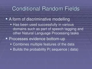
Conditional Random Fields. Probabilistic Graphical Models (10-708) Ramesh Nallapati. Y 1. Y 2. …. …. …. Y n. X 1. X 2. …. …. …. X n. Motivation: Shortcomings of Hidden Markov Model. HMM models direct dependence between each state and only its corresponding observation


Conditional Random Fields
E N D
Presentation Transcript
Conditional Random Fields Probabilistic Graphical Models (10-708) Ramesh Nallapati
Y1 Y2 … … … Yn X1 X2 … … … Xn Motivation:Shortcomings of Hidden Markov Model • HMM models direct dependence between each state and only its corresponding observation • NLP example: In a sentence segmentation task, segmentation may depend not just on a single word, but also on the features of the whole line such as line length, indentation, amount of white space, etc. • Mismatch between learning objective function and prediction objective function • HMM learns a joint distribution of states and observations P(Y, X), but in a prediction task, we need the conditional probability P(Y|X)
Y1 Y2 … … … Yn X1:n Solution:Maximum Entropy Markov Model (MEMM) • Models dependence between each state and the full observation sequence explicitly • More expressive than HMMs • Discriminative model • Completely ignores modeling P(X): saves modeling effort • Learning objective function consistent with predictive function: P(Y|X)
MEMM: Label bias problem Observation 1 Observation 2 Observation 3 Observation 4 0.4 0.45 0.5 State 1 0.2 0.2 0.1 0.6 0.55 0.5 0.2 0.3 0.3 State 2 0.2 0.1 0.2 State 3 0.2 0.1 0.2 State 4 0.2 0.3 0.2 State 5 • What the local transition probabilities say: • State 1 almost always prefers to go to state 2 • State 2 almost always prefer to stay in state 2
MEMM: Label bias problem Observation 1 Observation 2 Observation 3 Observation 4 0.45 0.5 0.4 State 1 0.2 0.2 0.1 0.6 0.55 0.5 0.2 0.3 0.3 State 2 0.2 0.1 0.2 State 3 0.2 0.1 0.2 State 4 0.2 0.3 0.2 State 5 • Probability of path 1-> 1-> 1-> 1: • 0.4 x 0.45 x 0.5 = 0.09
MEMM: Label bias problem Observation 1 Observation 2 Observation 3 Observation 4 0.45 0.5 0.4 State 1 0.2 0.2 0.1 0.6 0.55 0.5 0.2 0.3 0.3 State 2 0.2 0.1 0.2 State 3 0.2 0.1 0.2 State 4 0.2 0.3 0.2 State 5 • Probability of path 2->2->2->2 : • 0.2 X 0.3 X 0.3 = 0.018 Other paths: 1-> 1-> 1-> 1: 0.09
MEMM: Label bias problem Observation 1 Observation 2 Observation 3 Observation 4 0.45 0.5 0.4 State 1 0.2 0.2 0.1 0.6 0.55 0.5 0.2 0.3 0.3 State 2 0.2 0.1 0.2 State 3 0.2 0.1 0.2 State 4 0.2 0.3 0.2 State 5 • Probability of path 1->2->1->2: • 0.6 X 0.2 X 0.5 = 0.06 Other paths: 1->1->1->1: 0.09 2->2->2->2: 0.018
MEMM: Label bias problem Observation 1 Observation 2 Observation 3 Observation 4 0.45 0.5 0.4 State 1 0.2 0.2 0.1 0.6 0.55 0.5 0.2 0.3 0.3 State 2 0.2 0.1 0.2 State 3 0.2 0.1 0.2 State 4 0.2 0.3 0.2 State 5 • Probability of path 1->1->2->2: • 0.4 X 0.55 X 0.3 = 0.066 Other paths: 1->1->1->1: 0.09 2->2->2->2: 0.018 1->2->1->2: 0.06
MEMM: Label bias problem Observation 1 Observation 2 Observation 3 Observation 4 0.45 0.5 0.4 State 1 0.2 0.2 0.1 0.6 0.55 0.5 0.2 0.3 0.3 State 2 0.2 0.1 0.2 State 3 0.2 0.1 0.2 State 4 0.2 0.3 0.2 State 5 • Most Likely Path: 1-> 1-> 1-> 1 • Although locally it seems state 1 wants to go to state 2 and state 2 wants to remain in state 2. • why?
MEMM: Label bias problem Observation 1 Observation 2 Observation 3 Observation 4 0.45 0.5 0.4 State 1 0.2 0.2 0.1 0.6 0.55 0.5 0.2 0.3 0.3 State 2 0.2 0.1 0.2 State 3 0.2 0.1 0.2 State 4 0.2 0.3 0.2 State 5 • Most Likely Path: 1-> 1-> 1-> 1 • State 1 has only two transitions but state 2 has 5: • Average transition probability from state 2 is lower
MEMM: Label bias problem Observation 1 Observation 2 Observation 3 Observation 4 0.45 0.5 0.4 State 1 0.2 0.2 0.1 0.6 0.55 0.5 0.2 0.3 0.3 State 2 0.2 0.1 0.2 State 3 0.2 0.1 0.2 State 4 0.2 0.3 0.2 State 5 • Label bias problem in MEMM: • Preference of states with lower number of transitions over others
Solution: Do not normalize probabilities locally Observation 1 Observation 2 Observation 3 Observation 4 0.4 0.45 0.5 State 1 0.2 0.2 0.1 0.6 0.55 0.5 0.2 0.3 0.3 State 2 0.2 0.1 0.2 State 3 0.2 0.1 0.2 State 4 0.2 0.3 0.2 State 5 From local probabilities ….
Solution: Do not normalize probabilities locally Observation 1 Observation 2 Observation 3 Observation 4 20 30 5 State 1 10 20 10 30 20 5 20 30 30 State 2 10 10 20 State 3 20 10 20 State 4 20 30 20 State 5 • From local probabilities to local potentials • States with lower transitions do not have an unfair advantage!
Y1 Y2 … … … Yn X1:n From MEMM ….
Y1 Y2 … … … Yn x1:n From MEMM to CRF • CRF is a partially directed model • Discriminative model like MEMM • Usage of global normalizer Z(x) overcomes the label bias problem of MEMM • Models the dependence between each state and the entire observation sequence (like MEMM)
Y1 Y2 … … … Yn x1:n Conditional Random Fields • General parametric form:
Y1 Y2 … … … Yn x1:n Yn-1,Yn Y1,Y2 Y2,Y3 ……. Yn-2 Yn-2,Yn-1 Yn-1 Y2 Y3 CRFs: Inference • Given CRF parameters and , find the y* that maximizes P(y|x) • Can ignore Z(x) because it is not a function of y • Run the max-product algorithm on the junction-tree of CRF: Same as Viterbi decoding used in HMMs!
CRF learning • Given {(xd, yd)}d=1N, find *, * such that • Computing the gradient w.r.t : Gradient of the log-partition function in an exponential family is the expectation of the sufficient statistics.
CRF learning • Computing the model expectations: • Requires exponentially large number of summations: Is it intractable? • Tractable! • Can compute marginals using the sum-product algorithm on the chain Expectation of f over the corresponding marginal probability of neighboring nodes!!
Y1 Y2 … … … Yn x1:n CRF learning • Computing marginals using junction-tree calibration: • Junction Tree Initialization: • After calibration: Yn-1,Yn Y1,Y2 Y2,Y3 ……. Yn-2 Yn-2,Yn-1 Yn-1 Y2 Y3 Also called forward-backward algorithm
CRF learning • Computing feature expectations using calibrated potentials: • Now we know how to compute rL(,): • Learning can now be done using gradient ascent:
CRF learning • In practice, we use a Gaussian Regularizer for the parameter vector to improve generalizability • In practice, gradient ascent has very slow convergence • Alternatives: • Conjugate Gradient method • Limited Memory Quasi-Newton Methods
CRFs: some empirical results • Comparison of error rates on synthetic data MEMM error MEMM error HMM error CRF error Data is increasingly higher order in the direction of arrow CRF error CRFs achieve the lowest error rate for higher order data HMM error
CRFs: some empirical results • Parts of Speech tagging • Using same set of features: HMM >=< CRF > MEMM • Using additional overlapping features: CRF+ > MEMM+ >> HMM
Other CRFs • So far we have discussed only 1-dimensional chain CRFs • Inference and learning: exact • We could also have CRFs for arbitrary graph structure • E.g: Grid CRFs • Inference and learning no longer tractable • Approximate techniques used • MCMC Sampling • Variational Inference • Loopy Belief Propagation • We will discuss these techniques in the future
Summary • Conditional Random Fields are partially directed discriminative models • They overcome the label bias problem of MEMMs by using a global normalizer • Inference for 1-D chain CRFs is exact • Same as Max-product or Viterbi decoding • Learning also is exact • globally optimum parameters can be learned • Requires using sum-product or forward-backward algorithm • CRFs involving arbitrary graph structure are intractable in general • E.g.: Grid CRFs • Inference and learning require approximation techniques • MCMC sampling • Variational methods • Loopy BP