Reasoning Under Uncertainty: Handling Probabilistic Knowledge in Belief Networks
280 likes | 406 Vues
This document covers the essential aspects of reasoning under uncertainty, focusing on handling uncertain knowledge through probability theory and belief networks. It discusses the limitations of deterministic rules in medical diagnosis, illustrates the use of Bayes’ Rule, and explains how belief networks represent joint probability distributions and conditional independence. The application of these concepts is exemplified with realistic scenarios like burglar alarm systems and car ignition functions, highlighting the mechanics of inference in uncertain environments.

Reasoning Under Uncertainty: Handling Probabilistic Knowledge in Belief Networks
E N D
Presentation Transcript
Reasoning under Uncertainty Department of Computer Science & Engineering Indian Institute of Technology Kharagpur
Handling uncertain knowledge • p Symptom(p, Toothache) Disease(p, Cavity) • Not correct, since toothache can be caused in many other cases • p Symptom(p, Toothache) Disease(p, Cavity) Disease(p, GumDisease) Disease(p, ImpactedWisdom) … • p Disease(p, Cavity) Symptom(p, Toothache) • This is not correct either, since all cavities do not cause toothache
Reasons for using probability • Laziness • It is too much work to list the complete set of antecedents or consequents needed to ensure an exception-less rule • Theoretical ignorance • The complete set of antecedents is not known • Practical ignorance • The truth of the antecedents is not known, but we still wish to reason
Axioms of Probability • All probabilities are between 0 and 1: 0 P(A) 1 • P(True) = 1 and P(False) = 0 • P(A B) = P(A) + P(B) – P(A B) • Bayes’ Rule • P(A B) = P(A | B) P(B) • P(A B) = P(B | A) P(A)
Belief Networks A belief network is a graph in which the following holds: • A set of random variables makes up the nodes of the network • A set of random directed links or arrows connects pairs of nodes. The intuitive meaning of an arrow from node X to node Y is that X has a direct influence on Y • Each node has a conditional probability table that quantifies the effects that the parent have on the node. • The graph has no directed cycles (it is a DAG)
Example • Burglar alarm at your home • Fairly reliable at detecting a burglary • Also responds on occasion to minor earthquakes • Two neighbors who, on hearing the alarm calls you at office • John always calls when he hears the alarm, but sometimes confuses the telephone ringing with the alarm and calls then, too. • Mary likes loud music and sometimes misses the alarm altogether
Belief Network for the example Burglary Earthquake Alarm JohnCalls MaryCalls
Representing the joint probability distribution • A generic entry in the joint probability distribution P(x1, …, xn) is given by: • Probability of the event that the alarm has sounded but neither a burglary nor an earthquake has occurred, and both Mary and John call: P(J M A B E) = P(J | A) P(M | A) P(A | B E) P(B) P(E) = 0.9 X 0.7 X 0.001 X 0.999 X 0.998 = 0.00062
Conditional independence The belief network represents conditional independence:
Incremental Network Construction • Choose the set of relevant variables Xi that describe the domain • Choose an ordering for the variables (very important step) • While there are variables left: • Pick a variable X and add a node to the network for it • Set Parents(X) to some minimal set of nodes already in the net such that the conditional independence property is satisfied • Define the conditional probability table for X
Conditional Independence Relations • If every undirected path from a node in X to a node in Y is d-separated by a given set of evidence nodes E, then X and Y are conditionally independent given E. • A set of nodes E d-separates two sets of nodes X and Y if every undirected path from a node in X to a node in Y is blocked given E. • A path is blocked given a set of nodes E if there is a node Z on the path for which one of three conditions holds: • Z is in E and Z has one arrow on the path leading in and one arrow out • Z is in E and Z has both path arrows leading out • Neither Z nor any descendant of Z is in E, and both path arrows lead in to Z
Conditional Independence in belief networks Battery Petrol Radio Ignition Starts • Whether there is petrol and whether the radio plays are independent • given evidence about whether the ignition takes place • Petrol and Radio are independent if it is known whether the battery works • Petrol and Radio are independent given no evidence at all. But they are • dependent given evidence about whether the car starts. If the car does • not start, then the radio playing is increased evidence that we are out of • petrol.
Inferences using belief networks • Diagnostic inferences (from effects to causes) • Given that JohnCalls, infer that P(Burglary | JohnCalls) = 0.016 • Causal inferences (from causes to effects) • Given Burglary, P(JohnCalls | Burglary) = 0.86 and P(MaryCalls | Burglary) = 0.67 • Intercausal inferences (between causes of a common effect) • Given Alarm, we have P(Burglary | Alarm) = 0.376. But if we add the evidence that Earthquake is true, then P(Burglary | Alarm Earthquake) goes down to 0.003 • Mixed inferences (combining two or more of the above) • Setting the effect JohnCalls to true and the cause Earthquake to false gives P(Alarm | JohnCalls Earthquake) = 0.003
The four patterns Q E Q E E Q E Q E Causal InterCausal Mixed Diagnostic
An algorithm for answering queries • We consider cases where the belief network is a poly-tree • There is at most one undirected path between any two nodes • U = U1 … Um are • parents of node X • Y = Y1 … Yn are • children of node X • X is the query variable • E is a set of evidence • variables • The aim is to compute • P(X | E) U1 Um X Z1j Znj Y1 Yn
Definitions • EX+ is the causal support for X • The evidence variables “above” X that are connected to X through its parents • EX– is the evidential support for X • The evidence variables “below” X that are connected to X through its children • EUi \ Xrefers to all the evidence connected to node Ui except via the path from X • EYi \ X+refers to all the evidence connected to node Yi through its parents for X
The computation of P(X|E) • Since X d-separates EX+ from EX– in the network, we can use conditional • independence to simplify the first term in the numerator • We can treat the denominator as a constant
The computation of P(X | EX+) • We consider all possible configurations of the parents of X and how likely • they are given EX+. Let U be the vector of parents U1, …, Um, and let u be • an assignment of values to them. • Now U d-separates X from EX+, so we can simplify the first term to P(X | u) • We can simplify the second term by noting that EX+ d-separates each Ui from • the others, and that the probability of a conjunction of independent variables • is equal to the product of their individual probabilities
The computation of P(X | EX+) .. Contd… • The last term can be simplified by partitioning EX+ into EU1\X, …, EUm\X • and using the fact that EUi\X d-separates Ui from all the other evidence • in EX+ • P(X | u) is a lookup in the conditional probability table of X • P(ui | EUi\X) is a recursive (smaller) instance of the original problem
The computation of P(EX– | X) • Let Zi be the parents of Yi other than X, and let zi be an assignment of • of values to the parents • The evidence in each Yi box is conditionally independent of the others • given X • Averaging over Yi and zi yields: • Breaking EYi\X into the two independent components EYi– and EYi\X+
The computation of P(EX– | X) … contd • EYi– is independent of X and zi given yi, and EYi\X+is independent of X and yi • Apply Bayes’ rule to P(EYi\X+ | zi): • Rewriting the conjunction of Yi and zi:
The computation of P(EX– | X) … contd • P(zi | X) = P(zi) because Z and X are d-separated. Also P(EYi\X+) is a constant • The parents of Yi (the Zij) are independent of each other. • We also combine the i into one single
The computation of P(EX– | X) … contd • P(EYi– | yi) is a recursive instance of P(EX– | X) • P(yi | X, zi) is a conditional probability table entry for Yi • P(zij | EZij\Yi) is a recursive instance of the P(X | E) calculation
Inference in multiply connected belief networks • Clustering methods • Transform the network into a probabilistically equivalent (but topologically different) poly-tree by merging offending nodes • Conditioning methods • Instantiate variables to definite values, and then evaluate a poly-tree for each possible instantiation • Stochastic simulation methods • Use the network to generate a large number of concrete models of the domain that are consistent with the network distribution. • They give an approximation of the exact evaluation.
Default reasoning • Some conclusions are made by default unless a counter-evidence is obtained • Non-monotonic reasoning • Points to ponder • What is the semantic status of default rules? • What happens when the evidence matches the premises of two default rules with conflicting conclusions? • Sometimes a system may draw a number of conclusions on the basis of a belief that is later retracted. How can a system keep track of which conclusions need to be retracted as a result?
Rule-based methods for uncertain reasoning Issues: • Locality • In logical reasoning systems, if we have A B, then we can conclude B given evidence A, without worrying about any other rules. In probabilistic systems, we need to consider all available evidence. • Detachment • Once a logical proof is found for proposition B, we can use it regardless of how it was derived (it can be detached from its justification). In probabilistic reasoning, the source of the evidence is important for subsequent reasoning. • Truth functionality • In logic, the truth of complex sentences can be computed from the truth of the components. Probability combination does not work this way, except under strong independence assumptions. The most famous example of a truth functional system for uncertain reasoning is the certainty factors model, developed for the Mycin medical diagnostic program
Dempster-Shafer Theory • Designed to deal with the distinction between uncertainty and ignorance. • We use a belief function Bel(X) – probability that the evidence supports the proposition • When we do not have any evidence about X, we assign Bel(X) = 0 as well as Bel(X) = 0 For example, if we do not know whether a coin is fair, then: Bel( Heads ) = Bel( Heads ) = 0 If we are given that the coin is fair with 90% certainty, then: Bel( Heads ) = 0.9 X 0.5 = 0.45 Bel(Heads ) = 0.9 X 0.5 = 0.45 Note that we still have a gap of 0.1 that is not accounted for by the evidence
Fuzzy Logic • Fuzzy set theory is a means of specifying how well an object satisfies a vague description • Truth is a value between 0 and 1 • Uncertainty stems from lack of evidence, but given the dimensions of a man concluding whether he is fat has no uncertainty involved • The rules for evaluating the fuzzy truth, T, of a complex sentence are T(A B) = min( T(A), T(B) ) T(A B) = max( T(A), T(B) ) T(A) = 1 T(A)