Download
1 / 40
420 likes | 494 Vues
Explore the potential applications and limitations of Quantum Boltzmann Machines in machine learning. Discover the training techniques, properties, and insights into utilizing quantum annealers for sampling. Dive into the world of quantum computing and its integration with classical models.

E N D
Quantum Boltzmann Machine Mohammad Amin D-Wave Systems Inc.
Not the only use of QA Maybe not the best use of QA
Adiabatic Quantum Computation H(t) = (1-s)HD + sHP , s = t/tf energy levels gmin Solution Initial state 1 s 0 tf~ (1/gmin)2
Thermal Noise System Bath Interaction energy levels kBT P0 1 s 0 Dynamical freeze-out
Open quantum calculations of a 16 qubit random problem Classical energies
Equilibration Can Cause Correlation Correlation with simulated annealing Hen et al., PRA 92, 042325 (2015)
Equilibration Can Cause Correlation Correlation with Quantum Monte Carlo Boixo et al., Nature Phys. 10, 218 (2014)
Equilibration Can Cause Correlation Correlation with spin vector Monte Carlo Shin et al., arXiv:1401.7087 SVMC SVMC
Equilibration Can Mask Quantum Speedup Brooke et al., Science 284, 779 (1999) Quantum advantage is expected to be dynamical
Equilibration Can Mask Quantum Speedup Ronnow et al., Science 345, 420 (2014) Hen et al., arXiv:1502.01663 King et al., arXiv:1502.02098 Equilibrated probability!!! Computation time is independent of dynamics!
Residual Energy vs Annealing Time 50 random problems, 100 samples per problem per annealing time Bimodal (J=-1, +1 , h=0) Mean residual energy Lowest residual energy Annealing time (ms)
Residual Energy vs Annealing Time 50 random problems, 100 samples per problem per annealing time Frustrated loops (a=0.25) Bimodal (J=-1, +1 , h=0) Annealing time (ms) Annealing time (ms)
Boltzmann sampling is #P harder than NP What can we do with a QuantumBoltzmann Distribution?
arXiv:1601.02036 Bohdan Kulchytskyy Roger Melko Jason Rolfe Evgeny Andriyash
Introduction to Machine Learning Data Model 3 Unseen data Model
Probabilistic Models Data Probability distribution Variables Parameters q Model Training: Tune qsuch that
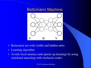
Boltzmann Machine Data Variables Parameters q Model Boltzmann distribution (b =1)
Boltzmann Machine Ising model: spins parameters
Adding Hidden Variables z i zn za=(zn ,zi) visible visiblehidden hidden
Training a BM Maximize log-likelihood: Or minimize: training rate gradient descent technique We need an efficient way to calculate Tune such that
Calculating the Gradient Unclamped average Average with clamped visibles
Training Ising Hamiltonian Parameters Clamped average Unclamped average Gradients can be estimated using sampling!
Question: Is it possible to train a quantum Boltzmann machine? Transverse Ising Hamiltonian Ising Hamiltonian
Quantum Boltzmann Distribution Boltzmann probability distribution: Density matrix: Identity matrix Projection operator
Gradient Descent = Classically: = Clamped average Unclamped average
Calculating the Gradient ≠ ≠ Clamped average Unclamped average Gradient cannot be estimated using sampling!
Two Useful Properties of Trace Golden-Thompson inequality: For Hermitian matrices A and B
Finding lower bounds Golden-Thompson inequality
Finding lower bounds Golden-Thompson inequality Lower bound for log-likelihood
Calculating the Gradients Minimize the upper bound ? Unclamped average
Clamped Hamiltonian for Infinite energy penalty for states different from v Visible qubits are clamped to their classical values given by the data
Estimating the Steps Clamped average Unclamped average We can now use sampling to estimate the steps
Training the Transverse Field (Ga) Minimizing the upper bound: Two problems: cannot be estimated from measurements for all visible qubits, thus Gn cannot be trained using the bound
Example: 10-Qubit QBM Graph: fully connected (K10), fully visible
Example: 10-Qubit QBM Training set: M-modal distribution Random spin orientation Hamming distance Multi-mode: Single mode: M = 8 p = 0.9
Exact Diagonalization Results KL-divergence: Bound gradient D=2 Classical BM Exact gradient (D is trained) D final= 2.5
Sampling from D-Wave Dickson et al., Nat. Commun. 4, 1903 (2013) Probabilities cross at the anticrossing
Conclusions: • A quantum annealer can provide fast samples of quantum Boltzmann distribution • QBM can be trained by sampling • QBM may learn some distributions better than classical BM • SeearXiv:1601.02036