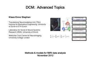
DCM: Advanced Topics
DCM: Advanced Topics. Klaas Enno Stephan Translational Neuromodeling Unit (TNU) Institute for Biomedical Engineering, University of Zurich & ETH Zurich Laboratory for Social & Neural Systems Research (SNS), University of Zurich

DCM: Advanced Topics
E N D
Presentation Transcript
DCM: Advanced Topics Klaas Enno Stephan Translational Neuromodeling Unit (TNU)Institute for Biomedical Engineering, University of Zurich & ETH Zurich Laboratory for Social & Neural Systems Research (SNS), University of Zurich WellcomeTrust Centre for Neuroimaging, University College London Methods & models for fMRI data analysisNovember 2012
Overview • Bayesianmodelselection (BMS) • Extended DCM forfMRI: nonlinear, two-state, stochastic • Embedding computational models in DCMs • Integratingtractographyand DCM • ApplicationsofDCM toclinicalquestions
Dynamic Causal Modeling (DCM) Hemodynamicforward model:neural activityBOLD Electromagnetic forward model:neural activityEEGMEG LFP Neural state equation: fMRI EEG/MEG simple neuronal model complicated forward model complicated neuronal model simple forward model inputs
Generative models & model selection • any DCM = a particular generative model of how the data (may) have been caused • modelling = comparing competing hypotheses about the mechanisms underlyingobserveddata • a priori definitionofhypothesisset (modelspace) iscrucial • determinethemost plausible hypothesis (model), giventhedata • model selection model validation! • model validation requires external criteria (external to the measured data)
Pitt & Miyung (2002) TICS Model comparison and selection Given competing hypotheses on structure & functional mechanisms of a system, which model is the best? Which model represents thebest balance between model fit and model complexity? For which model m does p(y|m) become maximal?
Bayesian model selection (BMS) Model evidence: Gharamani, 2004 p(y|m) accounts for both accuracy and complexity of the model y all possible datasets allows for inference about structure (generalisability) of the model • Various approximations, e.g.: • negative free energy, AIC, BIC McKay 1992, Neural Comput. Penny et al. 2004a, NeuroImage
Approximations to the model evidence in DCM Maximizing log model evidence = Maximizing model evidence Logarithm is a monotonic function Log model evidence = balance between fit and complexity No. of parameters SPM2 & SPM5 offered 2 approximations: No. of data points Akaike Information Criterion: Bayesian Information Criterion: Penny et al. 2004a, NeuroImage Penny 2012, NeuroImage
The (negative) free energy approximation • UnderGaussianassumptionsabouttheposterior (Laplace approximation):
The complexity term in F • In contrastto AIC & BIC, thecomplexitytermofthe negative freeenergyFaccountsforparameterinterdependencies. • The complexitytermofFishigher • themoreindependentthepriorparameters ( effective DFs) • themoredependenttheposteriorparameters • themoretheposteriormeandeviatesfromthepriormean • NB: Since SPM8, onlyFisusedformodelselection !
Bayes factors To compare two models, we could just compare their log evidences. But: the log evidence is just some number – not very intuitive! A more intuitive interpretation of model comparisons is made possible by Bayes factors: positive value, [0;[ Kass & Raftery classification: Kass & Raftery 1995, J. Am. Stat. Assoc.
M3 attention M2 better than M1 PPC BF 2966 F = 7.995 stim V1 V5 M4 attention PPC stim V1 V5 BMS in SPM8: an example attention M1 M2 PPC PPC attention stim V1 V5 stim V1 V5 M3 M1 M4 M2 M3 better than M2 BF 12 F = 2.450 M4 better than M3 BF 23 F = 3.144
Fixed effects BMS at group level Group Bayes factor (GBF) for 1...K subjects: Average Bayes factor (ABF): Problems: • blind with regard to group heterogeneity • sensitive to outliers
Random effects BMS forheterogeneousgroups Dirichlet parameters = “occurrences” of models in the population Dirichlet distribution of model probabilities r Multinomial distribution of model labels m Model inversion by VariationalBayes (VB) or MCMC Measured data y Stephan et al. 2009a, NeuroImage Penny et al. 2010, PLoS Comp. Biol.
LD LD|LVF LD|RVF LD|LVF LD LD RVF stim. LD LVF stim. RVF stim. LD|RVF LVF stim. MOG MOG MOG MOG LG LG LG LG FG FG FG FG m2 m1 m2 m1 Data: Stephan et al. 2003, Science Models: Stephan et al. 2007, J. Neurosci.
m2 m1 Stephan et al. 2009a, NeuroImage
Model space partitioning: comparing model families m2 m1 m2 m1 Stephan et al. 2009, NeuroImage
Comparing model families – a second example • data from Leff et al. 2008, J. Neurosci • one driving input, one modulatory input • 26 = 64 possible modulations • 23 – 1 input patterns • 764 = 448 models • integrate out uncertainty about modulatory patterns and ask where auditory input enters Penny et al. 2010, PLoS Comput. Biol.
Bayesian Model Averaging (BMA) • abandons dependence of parameter inference on a single model • uses the entire model space considered (or an optimal family of models) • computes average of each parameter, weighted by posterior model probabilities • represents a particularly useful alternative • when none of the models (or model subspaces) considered clearly outperforms all others • when comparing groups for which the optimal model differs NB: p(m|y1..N) can be obtained by either FFX or RFX BMS Penny et al. 2010, PLoS Comput. Biol.
definition of model space inference on model structure or inference on model parameters? inference on individual models or model space partition? inference on parameters of an optimal model or parameters of all models? optimal model structure assumed to be identical across subjects? comparison of model families using FFX or RFX BMS optimal model structure assumed to be identical across subjects? BMA yes no yes no FFX BMS RFX BMS FFX BMS RFX BMS FFX analysis of parameter estimates (e.g. BPA) RFX analysis of parameter estimates (e.g. t-test, ANOVA) Stephan et al. 2010, NeuroImage
Overview • Bayesianmodelselection (BMS) • Extended DCM forfMRI: nonlinear, two-state, stochastic • Embedding computational models in DCMs • Integratingtractographyand DCM • Applicationsof DCM toclinicalquestions
DCM10 in SPM8 • DCM10 was released as part of SPM8 in July 2010 (version 4010). • Introduced many new features, incl. two-state DCMs and stochastic DCMs • This led to various changes in model defaults, e.g. • inputs mean-centred • changes in coupling priors • self-connections estimatedseparatelyfor each area • For details, see: www.fil.ion.ucl.ac.uk/spm/software/spm8/SPM8_Release_Notes_r4010.pdf • Further changes in version 4290 (released April 2011) to accommodate new developments and give users more choice (e.g., whether or not to mean-centre inputs).
The evolution of DCM in SPM • DCM is not one specific model, but a framework for Bayesian inversion of dynamic system models • The default implementation in SPM is evolving over time • improvementsofnumericalroutines (e.g., forinversion) • change in priors to cover new variants (e.g., stochastic DCMs, endogenous DCMs etc.) To enable replication of your results, you should ideally state which SPM version (releasenumber) you are using when publishing papers. In thenext SPM version, thereleasenumber will bestored in theDCM.mat.
Neural state equation endogenous connectivity modulation of connectivity direct inputs modulatory input u2(t) driving input u1(t) t t y BOLD y y y λ hemodynamic model activity x2(t) activity x3(t) activity x1(t) x neuronal states integration The classical DCM: a deterministic, one-state, bilinear model
Factorial structure of model specification in DCM10 • Three dimensions of model specification: • bilinear vs. nonlinear • single-state vs. two-state (per region) • deterministic vs. stochastic • Specification via GUI.
non-linear DCM modulation driving input bilinear DCM driving input modulation Two-dimensional Taylor series (around x0=0, u0=0): Nonlinear state equation: Bilinear state equation:
Neural population activity x3 fMRI signal change (%) x1 x2 u2 u1 Nonlinear dynamic causal model (DCM) Stephan et al. 2008, NeuroImage
attention MAP = 1.25 0.10 PPC 0.26 0.39 1.25 0.26 V1 stim 0.13 V5 0.46 0.50 motion Stephan et al. 2008, NeuroImage
Two-state DCM Single-state DCM Two-state DCM input Extrinsic (between-region) coupling Intrinsic (within-region) coupling Marreiros et al. 2008, NeuroImage
Estimates of hidden causes and states (Generalised filtering) Stochastic DCM • all states are represented in generalised coordinates of motion • random state fluctuations w(x)account for endogenous fluctuations,have unknown precision and smoothness two hyperparameters • fluctuations w(v) induce uncertainty about how inputs influence neuronal activity • can be fitted to resting state data Li et al. 2011, NeuroImage
Overview • Bayesianmodelselection (BMS) • Extended DCM forfMRI: nonlinear, two-state, stochastic • Embedding computational models in DCMs • Integratingtractographyand DCM • Applicationsof DCM toclinicalquestions
Prediction errors drive synaptic plasticity PE(t) x3 R x1 x2 McLaren 1989 synaptic plasticity during learning = f (prediction error)
Conditioning Stimulus Target Stimulus or 1 0.8 or 0.6 CS TS Response 0.4 0 200 400 600 800 2000 ± 650 CS 1 Time (ms) CS 0.2 2 0 0 200 400 600 800 1000 Learning ofdynamic audio-visualassociations p(face) trial den Ouden et al. 2010, J. Neurosci.
k vt-1 vt rt rt+1 ut ut+1 Hierarchical Bayesian learning model prior on volatility volatility probabilistic association observed events Behrens et al. 2007, Nat. Neurosci.
1 True Bayes Vol HMM fixed 0.8 HMM learn RW 0.6 p(F) 450 0.4 440 0.2 430 RT (ms) 420 0 400 440 480 520 560 600 Trial 410 400 390 0.1 0.3 0.5 0.7 0.9 p(outcome) Explaining RTs by different learning models Reaction times Bayesian model selection: hierarchical Bayesianmodel performsbest • 5 alternative learning models: • categorical probabilities • hierarchical Bayesian learner • Rescorla-Wagner • Hidden Markov models (2 variants) den Ouden et al. 2010, J. Neurosci.
p < 0.05 (SVC) 0 0 -0.5 -0.5 BOLD resp. (a.u.) BOLD resp. (a.u.) -1 -1 -1.5 -1.5 -2 -2 p(F) p(H) p(F) p(H) Stimulus-independent prediction error Putamen Premotor cortex p < 0.05 (cluster-level whole- brain corrected) den Ouden et al. 2010, J. Neurosci.
Prediction error (PE) activity in the putamen PE duringactive sensorylearning PE duringincidental sensorylearning den Ouden et al. 2009, Cerebral Cortex p < 0.05 (SVC) PE during reinforcement learning PE = “teaching signal” for synaptic plasticity during learning O'Doherty et al. 2004, Science Could the putamen be regulating trial-by-trial changes of task-relevant connections?
Prediction errors control plasticity during adaptive cognition Hierarchical Bayesian learning model PUT • Influence of visual areas on premotor cortex: • stronger for surprising stimuli • weaker for expected stimuli p= 0.017 p= 0.010 PMd PPA FFA ongoingpharmacological andgeneticstudies den Ouden et al. 2010, J. Neurosci.
Hierarchical variational Bayesian learning volatility association events in the world sensory stimuli Mean-fielddecomposition Mathys et al. (2011), Front. Hum. Neurosci.
Overview • Bayesianmodelselection (BMS) • Extended DCM forfMRI: nonlinear, two-state, stochastic • Embedding computational models in DCMs • Integratingtractographyand DCM • Applicationsof DCM toclinicalquestions
Diffusion-weighted imaging Parker & Alexander, 2005, Phil. Trans. B
Integration of tractography and DCM R1 R2 low probability of anatomical connection small prior variance of effective connectivity parameter R1 R2 high probability of anatomical connection large prior variance of effective connectivity parameter Stephan, Tittgemeyer et al. 2009, NeuroImage
probabilistic tractography FG right LG right anatomicalconnectivity LG left FG left LG LG FG FG Proofofconceptstudy DCM connection-specificpriorsforcouplingparameters Stephan, Tittgemeyer et al. 2009, NeuroImage
Connection-specific prior variance as a function of anatomical connection probability • 64 different mappings by systematic search across hyper-parameters and • yields anatomically informed (intuitive and counterintuitive) and uninformed priors
Models with anatomically informed priors (of an intuitive form)
Models with anatomically informed priors (of an intuitive form) were clearly superiortoanatomically uninformed ones: Bayes Factor >109
Overview • Bayesian model selection (BMS) • Extended DCM for fMRI: nonlinear, two-state, stochastic • Embedding computational models in DCMs • Integrating tractography andDCM • Applicationsof DCM toclinicalquestions
Model-based predictions for single patients model structure BMS set of parameter estimates model-based decoding
BMS: Parkison‘s disease and treatment Age-matched controls PD patients on medication PD patients off medication Selection of action modulates connections between PFC and SMA DA-dependent functional disconnection of the SMA Rowe et al. 2010, NeuroImage
Model-based decoding by generative embedding A A step 1 — model inversion step 2 — kernel construction A → B A → C B → B B → C B B C C measurements from an individual subject subject-specificinverted generative model subject representation in the generative score space step 3 — support vector classification step 4 — interpretation jointly discriminative model parameters separating hyperplane fitted to discriminate between groups Brodersen et al. 2011, PLoS Comput. Biol.