Queueing Model for an Assemble-to-Order Manufacturing System- A Matrix Geometric Solution Approach
270 likes | 450 Vues
This paper presents a queueing model for a two-stage Assemble-to-Order (ATO) manufacturing system, focusing on understanding its dynamics and evaluating key performance measures. It discusses the system's structure, including demand arrival modeling, service rates, and inventory distribution. Utilizing matrix geometric methods, the paper provides exact solutions for various performance metrics such as order fulfillment time and work-in-process units. The aim is to enhance insights into ATO systems and explore optimization opportunities for improved efficiency.

Queueing Model for an Assemble-to-Order Manufacturing System- A Matrix Geometric Solution Approach
E N D
Presentation Transcript
Queueing Model for an Assemble-to-Order Manufacturing System- A Matrix Geometric Solution Approach Sachin Jayaswal Department of Management Sicences University of Waterloo Beth Jewkes Department of Management Sciences University of Waterloo
Outline • Motivation • Model Description • Literature Review • Analysis • Future Directions
Motivation • Get a better understanding of Assemble-to-Order (ATO) production systems • Develop a queuing model for a two stage ATO production system and evaluate the following measures of performance: • Distribution of semi-finished goods inventory • Distribution of order fulfillment time
Model Description λ Demand Arrival
Model Description Notations: • λ : demand rate (Poisson arrivals) • μj : service rate at stage j, j=1, 2 (exponential service times) • B1: base stock level at stage 1 (parameter) • N1: queue occupancy at stage 1 • N2: queue occupancy at stage 2 • I1 : semi-finished goods inventory after stage 1. I1 = [B1 – N1]+ • BO :Number of units backordered at stage 1. BO = [N1 – B1]+
Model Description If B1 = 0, the system is MTO and operates like an ordinary tandem queue: • The process describing the departure of units from each stage is Poisson with rate λ • Individual queues behave as if they are operated independently. In equilibrium, N1 and N2 are independent
Model Description • For the ATO with B1 > 0: • Arrival process to stage 2 is no longer poisson. • There is a positive dependence between the arrival of input units from stage 1 to stage 2. Times between successive arrivals to stage 2 are correlated.
Related Literature • Buzacott et al. (1992) observe that C.V. of inter-arrival times at stage 2 is between 0.8 and 1 and, therefore, recommend using an M/M/1 approximation for stage-2 queue. Lee and Zipkin (1992) also assume M/M/1 approximation for stage 2. (BPS-LZ approximation) • Buzacott et al. (1992) further improve upon this approximation by modeling the congestion at stage 2 as GI/M/1 queue. (BPS approximation) • Gupta and Benjaafar (2004) use BPS-LZ approximation to compare alternative MTS and MTO systems
Solution – Matrix Geometric Method State space representation 1 • Consider a finite queue before stage 2 with size k • State description: {N = (N1, N2) : N1 ≥ 0; 0 ≤ N2 ≤ k+1}
Infinitesimal Generator Q = This is a special case of a level dependent QBD
Solution… State space representation 2 • Consider a finite queue before stage 1 with size k • State description: {N = (N2, N1) : N2 ≥ 0; 0 ≤ N1 ≤ k+1}
Infinitesimal Generator Q is a level independent QBD process and hence can be solved using standard Matrix-Geometric Method Q =
An Exact Solution • The above methods are not truly exact as one of the queues is truncated • We next present an exact solution for the doubly infinite problem, using censoring (Grassmann & Standford (2000); Standford, Horn & Latouche (2005)) • State description: {N = (N2, N1) : N1 ≥ 0, N2 ≥ 0}
Censoring Infinitesimal Generator Q =
Censoring Transition Matrix: ; P =
P(1) = where Censoring Censoring all states above level 1 gives the following transition matrix: Censoring level 1 gives: P(0) infinite only in one dimension However, P(0) may no longer be QBD
Censoring R matrix: R = R matrix possesses asymptotically block Toeplitz form
Censoring P(0) = P(0) is also asymptotically of block Toeplitz form Hence, one can use GI/G/1 type Markov chains to study P(0)
Censoring GI/G/1 type Markov chain is of the form: P =
Censoring To make P(0) conform to GI/G/1 type Markov chain, we choose B0 to be sufficiently large to contain those elements not within a suitable tolerance of their asymptotic forms P(0) =
Censoring Transition matrix with all states beyond level n censored (Grassmann & Standford, 2000)
; ; t determined using generating function (Grassmann & Standford (2000)) Solution to level-0 probabilities Non-normalized probabilities αj for censored process Normalized probabilities for censored process
Solution Stationary vector at positive levels • Performance measures • EK2: Expected no. of units stage 2 still needs to produce to meet the pending demands. EK2 = E(N2+BO) • EI: Expected no. of work-in-process units. EI = E(I1+N2)
Initial Results λ=1; μ1 =1.25; μ2 =2
Future Directions • To construct an optimization model using the performance measures obtained • To compare the results obtained with the approximations suggested in the literature