Distance-Vector and Path-Vector Routing Sections 4.2.2., 4.3.2, 4.3.3

1. Distance-Vector and Path-Vector RoutingSections 4.2.2., 4.3.2, 4.3.3 COS 461: Computer Networks Spring 2011 Mike Freedman http://www.cs.princeton.edu/courses/archive/spring11/cos461/

2. Goals of Today’s Lectures • Distance-vector routing • Pro: Less information than link state • Con: Slower convergence • Path-vector routing • Faster convergence than distance vector • More flexibility in selecting paths • Different goals / metrics if inter- or intra-domain

3. Distance Vector: Still Shortest-Path Routing 2 1 3 1 4 2 1 5 4 3 • Path-selection model • Destination-based • Load-insensitive (e.g., static link weights) • Minimum hop count or sum of link weights

4. Shortest-Path Problem v (u,v) w (u,w) x (u,w) y (u,v) z (u,v) s (u,w) (u,w) t Ex) Forwarding table at u link 2 1 3 1 4 u 2 1 5 4 3 6 s • Compute: path costs to all nodes • From a given source u to all other nodes • Cost of the path through each outgoing link • Next hop along the least-cost path to s

5. Comparison of Protocols Link State Distance Vector Knowledge of neighbors’ distance to destinations Every router has O (#neighbors * #nodes) Trust a peer’s routing computation Use Bellman-Ford algorithm Send updates periodically or routing decision change Ex: RIP, IGRP Adv: Less info & lower computational overhead • Knowledge of every router’s links (entire graph) • Every router has O(# edges) • Trust a peer’s info, do routing computation yourself • Use Dijkstra’s algorithm • Send updates on any link-state changes • Ex: OSPF, IS-IS • Adv: Fast to react to changes

6. Bellman-Ford Algorithm 2 v y 1 3 1 4 x z u 2 1 5 t du(z) = min{ c(u,v) + dv(z), c(u,w) + dw(z) } w 4 3 s • Define distances at each node x • dx(y) = cost of least-cost path from x to y • Update distances based on neighbors • dx(y) = min {c(x,v) + dv(y)} over all neighbors v

7. Distance Vector Algorithm • Node x maintains state: • c(x,v) = cost for direct link from x to neighbor v • Distance vector Dx(y) (estimate of least cost x to y) for all nodes y • Distance vector Dv(y) for each neighbor v, for all y • Node x periodically sends Dx to its neighbors v • Neighbors update their own distance vectors: Dv(y) ← minx{c(v,x) + Dx(y)} for each node y ∊ N • Over time, the distance vector Dx converges

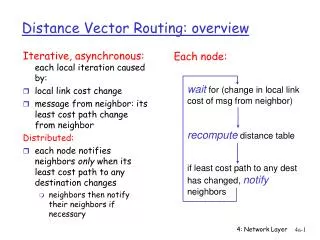
8. Iterative, asynchronous: Each local iteration by Local link cost change Distance vector update message from neighbor Distributed: Each node notifies neighbors only when its DV changes Neighbors then notify their neighbors if necessary Distance Vector Algorithm waitfor (change in local link cost or msg from neighbor) recompute estimates if distance to any destination has changed, notifyneighbors Each node:

9. Distance Vector Example: Step 1 Optimum 1-hop paths E C 3 1 1 F 2 6 1 3 D A 4 B

10. Distance Vector Example: Step 2 Optimum 2-hop paths E C 3 1 1 F 2 6 1 3 D A 4 B

11. Distance Vector Example: Step 3 Optimum 3-hop paths E C 3 1 1 F 2 6 1 3 D A 4 B

12. Distance Vector: Link Cost Changes 1 4 1 50 X Z Y • Link cost changes: • Node detects local link cost change • Updates the distance table • If cost change in least cost path, notify neighbors View of X (about neighbor y and z’s routing tables) “Good news travels fast” algorithm terminates Circled entry is least cost

13. Distance Vector: Link Cost Changes 60 4 1 50 X Z Y • Link cost changes: • Good news travels fast • Bad news travels slow - “count to infinity” problem! View of X (about neighbor y and z’s routing tables) algorithm continues on!

14. Distance Vector: Poison Reverse 60 4 1 50 X Z Y • If Z routes through Y to get to X : • Z tells Y its (Z’s) distance to X is infinite (so Y won’t route to X via Z) • Still, can have problems when more than 2 routers are involved View of X (about neighbor y and z’s routing tables) algorithm terminates

15. Routing Information Protocol (RIP) • Distance vector protocol • Nodes send distance vectors every 30 seconds • … or, when an update causes a change in routing • Link costs in RIP • All links have cost 1 • Valid distances of 1 through 15 • … with 16 representing infinity • Small “infinity”  smaller “counting to infinity” problem • RIP is limited to fairly small networks • E.g., used in the Princeton campus network

16. Comparison of LS and DV Routing Message complexity • LS: with n nodes, E links, O(nE) messages sent • DV: exchange between neighbors only Speed of Convergence • LS: relatively fast • DV: convergence time varies • May be routing loops • Count-to-infinity problem Robustness: what happens if router malfunctions? LS: • Node can advertise incorrect link cost • Each node computes only its own table DV: • DV node can advertise incorrect path cost • Each node’s table used by others (error propagates)

17. Similarities of LS and DV Routing • Shortest-path routing • Metric-based, using link weights • Routers share a common view of how good a path is • As such, commonly used inside an organization • RIP and OSPF are mostly used as intra-domain protocols • E.g., Princeton uses RIP, and AT&T uses OSPF • But the Internet is a “network of networks” • How to stitch the many networks together? • When networks may not have common goals • … and may not want to share information

18. Path-Vector Routing

19. Shortest-Path Routing is Restrictive NO National ISP1 National ISP2 YES Regional ISP1 Regional ISP3 Regional ISP2 Cust1 Cust3 Cust2 All traffic must travel on shortest paths All nodes need common notion of link costs Incompatible with commercial relationships

20. Link-State Routing is Problematic • Topology information is flooded • High bandwidth and storage overhead • Forces nodes to divulge sensitive information • Entire path computed locally per node • High processing overhead in a large network • Minimizes some notion of total distance • Works only if policy is shared and uniform • Typically used only inside an AS • E.g., OSPF and IS-IS

21. Distance Vector is on the Right Track • Advantages • Hides details of the network topology • Nodes determine only “next hop” toward the dest • Disadvantages • Minimizes some notion of total distance, which is difficult in an interdomain setting • Slow convergence due to the counting-to-infinity problem (“bad news travels slowly”) • Idea: extend the notion of a distance vector • To make it easier to detect loops

22. Path-Vector Routing 2 “d: path (2,1)” “d: path (1)” 3 1 data traffic data traffic d • Extension of distance-vector routing • Support flexible routing policies • Avoid count-to-infinity problem • Key idea: advertise the entire path • Distance vector: send distance metric per dest d • Path vector: send the entire path for each dest d

23. Faster Loop Detection 2 “d: path (2,1)” “d: path (1)” 3 1 “d: path (3,2,1)” • Node can easily detect a loop • Look for its own node identifier in the path • E.g., node 1 sees itself in the path “3, 2, 1” • Node can simply discard paths with loops • E.g., node 1 simply discards the advertisement

24. Flexible Policies 2 3 1 2 3 1 • Each node can apply local policies • Path selection: Which path to use? • Path export: Which paths to advertise? • Examples • Node 2 may prefer the path “2, 3, 1” over “2, 1” • Node 1 may not let node 3 hear the path “1, 2”

25. Conclusions • Distance-vector routing • Pro: Less information and computation than link state • Con: Slower convergence (e.g., count to infinity) • Path-vector routing • Share entire path, not distance: faster convergence • More flexibility in selecting paths • Different goals / metrics if inter- or intra-domain • Next week: BPG (path-vector protocol b/w ASes)