Download
1 / 42
450 likes | 798 Vues
Using the Lyapunov method to examine stability in nonlinear systems provides insights beyond linear analysis. Learn about linearization, Jacobian matrices, eigenvalues, and Lyapunov functions, with practical examples and applications. Discover how to determine stability when linearization is inconclusive.

E N D
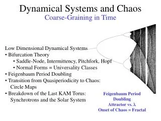
Dynamical Systems 3Nonlinear systems Ing. Jaroslav Jíra, CSc.
Stability of Nonlinear SystemsFirst Lyapunov method – linearization To examine stability of nonlinear systems we have to use more complicated tools than for linear ones. The first step, which frequently works, is the method of linearization, sometimes called first Lyapunov method. The principle is expanding of the right-hand side function in the equation of motion around the fixed point into the Taylor series with neglecting of higher order members. Taylor series Neglecting the higher order terms we obtain Being at an equilibrium point, we know, that f(x~)= dx~/dt = 0, so
Since the derivative of a constant is zero, then and consequently The original system Linearized system
Now we have to distinguish between the Jacobian matrix of the original system and the matrix for the linearized system at the specific fixed point, let’s say Df and Df(x~). While the Jacobian matrix of the original nonlinear system Df contains variables and constants, the Jacobian matrix of the linearized system at the fixed point Df(x~) contains just constants.
Example of the system linearization The system is defined by the set of equations To find the fixed points of the system, we have to solve equations We find two fixed points: Then we can do necessary calculations for the Jacobian matrix
Before examining stability of particular fixed points we can make a preview of the dynamical flow by the Mathematica program:
More detailed previews of areas around fixed points The area around the xA~ looks like a saddle point, i.e. the fixed point should be unstable The area around the xB~ looks like a sprial sink, i.e. the fixed point should be stable
Jacobian matrix of the original system is: For the first fixed point we have Eigenvalues of this matrix are approx. λ1=1.9016 and λ2= -1.4874 Conclusion: near xA~ the system behaves like a linear system with one positive and one negative eigenvalue, i.e. the system is unstablehere. For the second fixed point we have Eigenvalues of this matrix are approx. λ12= -1.2071 +/- 1.171i Conclusion: near xB~ the system behaves like a linear system with complex eigenvalues with negative real part, i.e. the system is stablehere.
What can we do if linearization method cannot decide? Example 2 – unusually damped harmonic oscillator We have a harmonic oscillator, where the mass m moves in very viscous medium, where the damping force is proportional to the cube of the velocity. Set of differential equations describing the system After setting vector variable y we can write Fixed point result from equations There is only one fixed point
The Jacobian matrix Jacobian matrix for linearized system at the fixed point Eigenvalues for this system are λ12= +/- i, so they have zero real part and the method of linearization cannot decide about the stability. The graph shows phase diagram for μ=0.25, x0=2 and v0=0. Even from the graph it is not clear if the trajectory will converge to (0,0) point or if it will remain at certain non-zero distance from it. We will have to use another tool – Lyapunov functions
Second Lyapunov method – Lyapunov functions If we look on the damped harmonic oscillator from the point of view of energy, there is clear, that the system is still losing energy and sooner or later it must stop at the equilibrium point (0,0). The principle of the second Lyapunov method is to find a function V(x) that represents energy or generalized energy and satisfies the following conditions. 1. the function V(x) is continuously differentiable around the fixed point 2. positive definiteV 3. negative definitedV/dt Additional condition to 3:at any state where the 3rd condition is considered satisfied if the system immediately moves to a state, where If we succeed in finding such function, then the fixed point x~ is stable.
Application of the second Lyapunov method on our Example 2 The total energy of a harmonic oscillator We simplify by taking m=1 and k=1 This function is continuously differentiable around zero and is positive for all states except for the fixed point (0,0), i.e. the first and second condition are satisfied. This means that we have a Lyapunov candidate function. The formula for the derivative of E
The final result for the time derivation is • We can notice that dE/dt is always negative except for the v=0, where dE/dt=0. The velocity is zero in three situations: • At the fixed point, which is in conformity with the third condition • At the instant, where the spring is maximally compressed • At the instant, where the spring is maximally extended • Situations 2 and 3 satisfy the additional condition, because the system immediately moves from here to the state where dE/dt<0. Also the third condition is satisfied. Conclusion: our Lyapunov candidate function satisfies all conditions for the Lyapunov function, so examined fixed point (0,0) is stable.
How to estimate Lyapunov candidate functions? If we examine a physical system, we should calculate the energy. If the state vector is xand the fixed point is 0, we could try If the fixed point is not at the origin of coordinate system, we have to modify If we are not successful, then we can try If it still does not work, we can use a general quadratic form
Classification of Stability of Nonlinear Systems 1. Lyapunov stability:fixed point x~ is a stable equilibrium if for every neighborhood U of x~ there is a neighborhood such that every solution x(t) starting in V remains in U for all times Lyapunov stability of an equilibrium means that solutions starting "close enough" to the equilibrium remain "close enough" forever. Such fixed point is considered Lyapunov stable or neutrally stable. In this case the third condition for Lyapunov function is satisfied, when dV/dt <=0. The time derivative must be negative semidefinite.
2. Asymptotic stability:fixed point x~ is asymptotically stable if it is Lyapunov stable and additionally V can be chosen so that for all Asymptotic stability means that solutions that start close enough not only remain close enough but also eventually converge to the equilibrium Such fixed point is considered asymptotically stable. In this case the third condition for Lyapunov function is satisfied, when dV/dt < 0. The time derivative must be negative definite.
3. Exponential stability:fixed point x~ is exponentially stable if there is a neighborhood V of x~ and a constant a>0 such that Exponential stability means that solutions not only converge, but in fact converge faster than or at least as fast as the exponential function Exp(-at). Exponentially stable equilibria are also asymptotically stable, and hence Lyapunov stable.
Bifurcations We distinguish two principal classes of bifurcations: Global bifurcation occurs when larger invariant sets of the system 'collide' with each other, or with equilibria of the system. They cannot be detected purely by a stability analysis of the equilibria (fixed points). The global bifurcation includes, for example, collision of a limit cycle with a saddle point, collision of a limit cycle with a node etc. Local bifurcation is a sudden change in the number or nature of the fixed and periodic points caused by a parameter change in the system. Fixed points may appear or disappear, change their stability, or even break apart into periodic points. Such bifurcation can be analysed entirely through changes in the local stability properties of equilibria, periodic orbits or other invariant sets.
The Logistic Equation The logistic equation, also known as Verhulst equation, is a formula for approximating the evolution of an animal population over time. Contrary to the bacteria model, living condition for animals significantly vary during the year. Some species are fertile just for particular season of year, not every existing animal reproduce etc. For this reason, the system might be better described by a discrete difference equation than a continuous differential equation. where xn is an actual population in the current year, xn+1 is population in the next year and r is combined rate for reproduction and for starvation. Zero value for the x means dead population and x=1 means population on its limit. Now we will examine what happens with stability and fixed points, if we try to change r. The only sure thing without any computations is, that for x(0)=0 we have a stable fixed point meaning dead population for any r.
Bifurcation diagram for the logistic equation The graph is an output of the Mathematica program. The initial value was x(0)=0.1 and 300 iterations were calculated for every r. For the value r=3 we can observe the first bifurcation (doubling of the functional dependence). Another bifurcations follow for r=3.449, r=3.544 etc.
The bifurcation diagram can be divided into 4 parts • Extinction(r<1): if the growth rate is less than 1 the system "dies„ • Fixed point area (1<r<3): the series tends to a single value for any initial x0 • Oscillation area (3<r<3.57): The series jumps between two or more discrete states. • Chaos area (3.57<r<4): the system can evaluate to any position at all with no apparent order • For higher values of r (r>4) all solutions zoom to infinity and the modeling aspects of this function become useless.
1. Saddle node (fold) bifurcation Differential equation of the system In this bifurcation two fixed points collide and annihilate each other. For r<0 there are two fixed points: a stable at and unstable at For r>0 there are no fixed points
Example for two-dimensional system, where r= -2 Differential equations Fixed points The Jacobian matrix Linearized Jacobian matrix for xA~ Eigenvalues for this Jacobian matrix Conclusion: the fixed point xA~ is a saddle point since there are real eigenvalues of various signs.
Linearized Jacobian matrix for xB~ Eigenvalues for this Jacobian matrix Conclusion: the fixed point xB~ is an attracting node since there are real eigenvalues, both of negative signs. The name of this bifurcation is derived from the pair of these two types of fixed points – saddle and node. __________________________________________________________________________________________________ An example of the saddle-node bifurcation for
2. Period doubling (flip) bifurcation This type of bifurcation can be observed at the logistic equation. If we accept also negative values, we observe period halving in the left part of the graph and period doubling in the right part.
3a. Pitchfork bifurcation Supercritical case In this bifurcation one fixed point splits into three various ones. Differential equation of the system Forr<0 there is just one stable fixed point at x=0 Forr>0 there is one unstable fixed point at x=0 and two stable fixed points at
3b. Pitchfork bifurcation Subcritical case In this bifurcation three various fixed points annihilate into one fixed point. Differential equation of the system Forr>0 there is just one unstable fixed point at x=0 Forr<0 there is one stable fixed point at x=0 and two unstable fixed points at
4. Transcritical bifurcation In this bifurcation there is one stable and one unstable fixed point and they exchange their stability when they collide. Differential equation of the system Forr<0 there is one stable fixed point at x=0 and one unstable fixed point for x=r Forr>0 there is one unstable fixed point at x=0 and one stable fixed point for x=r
5. Hopf bifurcation This bifurcation is a two-dimensional one. In this bifurcation a single fixed point changes into a limit cycle or vice versa. Differential equations of the system There is only one fixed point Jacobian matrix linearized Jacobian matrix
Eigenvalues determination Characteristic equation yields two complex conjugate roots According to our previous experience we can say, that for r<0 there is a stable fixed point and for r>0 there is an unstable fixed point. To be able to decide about r=0 we have to use a Lyapunov function, choosing candidate function We can clearly see, that for r=0 the dV/dt is outside the fixed point always negative, hence we have a Lyapunov function. This also tells us, that for r=0 the fixed point is Lyapunov stable and also asymptotically stable.
Phase diagram for r=-0.1, x10=1 and x20=0 Phase diagram for r=0, x10=1 and x20=0 Phase diagram for r=+0.1, x10=1 and x20=0 Phase diagram for r=+0.1, x10=0.2 and x20=0
3D interpretation of the Hopf Bifurcation. For negative values of r the system converges to the fixed point (0,0), for r=0 the system still converges to the fixed point, but very slowly. For positive values of r the attractor is not an unstable fixed point (0,0) but a limit cycle regardless of the starting point, i.e. it does not matter whether we start inside or outside the cycle. Diameter of the limit cycle raises with raising parameter r.
A program in Mathematica, which calculates the Hopf bifurcation
General rules concerning bifurcations. Continuous systems: a local bifurcation appears, when an eigenvalue has zero real part. If the eigenvalue is zero,then there is a saddle-node, pitchfork or transcritical bifurcation. If eigenvalues have zero real part, but they are complex conjugate, then there is a Hopf bifurcation. Discrete systems: a local bifurcation appears, when the modulus of eigenvalue is equal to one. If the eigenvalue is +1, then there is a saddle-node, pitchfork or transcritical bifurcation. If the eigenvalue is -1, then there is a period doubling bifurcation. If there are two complex conjugate eigenvalues with modulus equal to one, then there is a Hopf bifurcation.
Poincaré maps The Poincaré map, sometimes called first recurrence map, is the intersection of a periodic orbit in the phase space of a continuous dynamical system with a certain lower dimensional subspace, called the Poincaré section, transversal to the flow of the system. The method of Poincaré sections enables us to reduce multidimensional dynamical system by one or more dimensions and transforms continous function to a series of discrete points. In a simplified way we can say, that the Poincaré map is a profile of the phase portrait, where one or more state variables are constant.
Suppose we have a 3D plot Γ. Instead of directly studying the flow in 3D, we will examine the its intersection with a plane (x3=h) • Points of intersection in this case correspond to dx3/dt<0 • Height h of plane S is chosen so that Γcontinually crosses S. • The points P0, P1, P2 form the 2-D Poincaré section.
The following pictures illustrate distinguishing of various trajectories by their Poincaré sections. a) chaotic motion c) limit cycle b) stable fixed point d) cycle of period two
Example – we have a dynamical system described in cylindrical coordinates Solution of the equations -> 3D interpretation of the system λ<0 λ>0
A Poincaré map, constructed as a cut of the phase portrait by a halfplane Θ=0 looks like an attracting node for λ<0 and like a saddle point for λ>0. The point (x,z)=(0,1) corresponds to an intersection of the only closed orbit with the cutting halfplane. The second name of the Poincaré map – the first recurrence map means, that trajectories in the map consist of points, where xi is the actual intersection point of the trajectory and the plane, while xi+1 is the point, where the trajectory must return to the plane next time. First recurrence – first return. λ<0 λ>0
The explicite shape of our Poincaré map is where Tau=2*π/β is a period of the return to the cutting plane Continuous interpretation of the Poincaré sections from the Mathematica λ<0 λ>0