Download
1 / 24
280 likes | 592 Vues
Chapter 2. The Experimental Law of Coulomb. Coulomb’s Law and Electric Field Intensity. In 1600, Dr. Gilbert, a physician from England, published the first major classification of electric and non-electric materials.

E N D
Chapter 2 The Experimental Law of Coulomb Coulomb’s Law and Electric Field Intensity • In 1600, Dr. Gilbert, a physician from England, published the first major classification of electric and non-electric materials. • He stated that glass, sulfur, amber, and some other materials “not only draw to themselves straw, and chaff, but all metals, wood, leaves, stone, earths, even water and oil.” • In the following century, a French Army Engineer, Colonel Charles Coulomb, performed an elaborate series of experiments using devices invented by himself. • Coulomb could determine quantitatively the force exerted between two objects, each having a static charge of electricity. • He wrote seven important treatises on electric and magnetism, developed a theory of attraction and repulsion between bodies of the opposite and the same electrical charge.
Chapter 2 Coulomb’s Law and Electric Field Intensity The Experimental Law of Coulomb • Coulomb stated that the force between two very small objects separated in vacuum or free space by a distance which is large compared to their size is proportional to the charge on each and inversely proportional to the square of the distance between them. • In SI Units, the quantities of charge Q are measured in coulombs (C), the separation R in meters (m), and the force F should be newtons (N). • This will be achieved if the constant of proportionality k is written as:
Chapter 2 Coulomb’s Law and Electric Field Intensity The Experimental Law of Coulomb • The permittivity of free space ε is measured in farads per meter (F/m), and has the magnitude of: • The Coulomb’s law is now: • The force F acts along the line joining the two charges. It is repulsive if the charges are alike in sign and attractive if the are of opposite sign.
The Experimental Law of Coulomb Chapter 2 Coulomb’s Law and Electric Field Intensity • In vector form, Coulomb’s law is written as: • F2 is the force on Q2, for the case where Q1 and Q2 have the same sign, while a12 is the unit vector in the direction of R12, the line segment from Q1 to Q2.
Chapter 2 Coulomb’s Law and Electric Field Intensity The Experimental Law of Coulomb • Example • A charge Q1 = 310–4 C at M(1,2,3) and a charge of Q2 = –10–4 C at N(2,0,5) are located in a vacuum. Determine the force exerted on Q2 by Q1.
Chapter 2 Coulomb’s Law and Electric Field Intensity Electric Field Intensity • Let us consider one charge, say Q1, fixed in position in space. • Now, imagine that we can introduce a second charge, Qt, as a “unit test charge”, that we can move around. • We know that there exists everywhere a force on this second charge ►This second charge is displaying the existence of a force field. • The force on it is given by Coulomb’s law as: • Writing this force as a “force per unit charge” gives: Vector Field, Electric Field Intensity
Chapter 2 Coulomb’s Law and Electric Field Intensity Electric Field Intensity • We define the electric field intensity as the vector of force on a unit positive test charge. • Electric field intensity, E, is measured by the unit newtons per coulomb (N/C) or volts per meter (V/m). • The field of a single point charge can be written as: • aR is a unit vector in the direction from the point at which the point charge Q is located, to the point at which E is desired/measured.
Chapter 2 Coulomb’s Law and Electric Field Intensity Electric Field Intensity • For a charge which is not at the origin of the coordinate, the electric field intensity is:
Chapter 2 Coulomb’s Law and Electric Field Intensity Electric Field Intensity • The electric field intensity due to two point charges, say Q1 at r1 and Q2 at r2, is the sum of the electric field intensity on Qt caused by Q1 and Q2 acting alone (Superposition Principle).
Chapter 2 Coulomb’s Law and Electric Field Intensity Electric Field Intensity • Example A charge Q1 of 2 μC is located at at P1(0,0,0) and a second charge of 3 μC is at P2(–1,2,3). Find E at M(3,–4,2).
Chapter 2 Coulomb’s Law and Electric Field Intensity Field Due to a Continuous Volume Charge Distribution • We denote the volume charge density by ρv, having the units of coulombs per cubic meter (C/m3). • The small amount of charge ΔQ in a small volume Δv is • We may define ρv mathematically by using a limit on the above equation: • The total charge within some finite volume is obtained by integrating throughout that volume:
Chapter 2 Coulomb’s Law and Electric Field Intensity Field Due to a Continuous Volume Charge Distribution • Example • Find the total charge inside the volume indicated by ρv = 4xyz2, 0 ≤ ρ ≤ 2, 0 ≤ Φ ≤ π/2, 0 ≤ z ≤ 3. All values are in SI units.
Chapter 2 Coulomb’s Law and Electric Field Intensity Field Due to a Continuous Volume Charge Distribution • The contributions of all the volume charge in a given region, let the volume element Δv approaches zero, is an integral in the form of:
Chapter 2 Coulomb’s Law and Electric Field Intensity Field of a Line Charge • Now we consider a filamentlike distribution of volume charge density. It is convenient to treat the charge as a line charge of density ρL C/m. • Let us assume a straight-line charge extending along the z axis in a cylindrical coordinate system from –∞ to +∞. • We desire the electric field intensity E at any point resulting from a uniform line charge density ρL.
Chapter 2 Coulomb’s Law and Electric Field Intensity Field of a Line Charge • The incremental field dE only has the components in aρ and az direction, and no aΦ direction. • Why? • The component dEz is the result of symmetrical contributions of line segments above and below the observation point P. • Since the length is infinity, they are canceling each other ►dEz = 0. • The component dEρ exists, and from the Coulomb’s law we know that dEρ will be inversely proportional to the distance to the line charge, ρ.
Chapter 2 Coulomb’s Law and Electric Field Intensity Field of a Line Charge • Take P(0,y,0),
Chapter 2 Coulomb’s Law and Electric Field Intensity Field of a Line Charge • Now let us analyze the answer itself: • The field falls off inversely with the distance to the charged line, as compared with the point charge, where the field decreased with the square of the distance.
Chapter 2 Coulomb’s Law and Electric Field Intensity Field of a Line Charge • Example D2.5. • Infinite uniform line charges of 5 nC/m lie along the (positive and negative) x and y axes in free space. Find E at: (a) PA(0,0,4); (b) PB(0,3,4). PB PA • ρ is the shortest distance between an observation point and the line charge
Chapter 2 Coulomb’s Law and Electric Field Intensity Field of a Sheet of Charge • Another basic charge configuration is the infinite sheet of charge having a uniform density of ρS C/m2. • The charge-distribution family is now complete: point (Q), line (ρL), surface (ρS), and volume (ρv). • Let us examine a sheet of charge above, which is placed in the yz plane. • The plane can be seen to be assembled from an infinite number of line charge, extending along the z axis, from –∞ to +∞.
Chapter 2 Coulomb’s Law and Electric Field Intensity Field of a Sheet of Charge • For a differential width strip dy’, the line charge density is given by ρL = ρSdy’. • The component dEz at P is zero, because the differential segments above and below the y axis will cancel each other. • The component dEy at P is also zero, because the differential segments to the right and to theleft of z axis will cancel each other. • Only dEx is present, and this component is a function of x alone.
Chapter 2 Coulomb’s Law and Electric Field Intensity Field of a Sheet of Charge • The contribution of a strip to Ex at P is given by: • Adding the effects of all the strips,
Chapter 2 Coulomb’s Law and Electric Field Intensity Field of a Sheet of Charge • Fact: The electric field is always directed away from the positive charge, into the negative charge. • We now introduce a unit vector aN, which is normal to the sheet and directed away from it. • The field of a sheet of charge is constant in magnitude and direction. It is not a function of distance.
Chapter 1 Vector Analysis Homework 2 • D2.2. • D2.4. • D2.6. All homework problems from Hayt and Buck, 7th Edition. • Deadline: 25 January 2011, at 07:30.