Download
1 / 80
800 likes | 951 Vues
We can test the relationship between a quantitative dependent variable and two categorical independent variables with a two-factor analysis of variance (ANOVA). The two variables are referred to as “factors.”

E N D
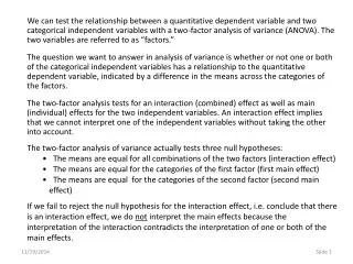
We can test the relationship between a quantitative dependent variable and two categorical independent variables with a two-factor analysis of variance (ANOVA). The two variables are referred to as “factors.” • The question we want to answer in analysis of variance is whether or not one or both of the categorical independent variables has a relationship to the quantitative dependent variable, indicated by a difference in the means across the categories of the factors. • The two-factor analysis tests for an interaction (combined) effect as well as main (individual) effects for the two independent variables. An interaction effect implies that we cannot interpret one of the independent variables without taking the other into account. • The two-factor analysis of variance actually tests three null hypotheses: • The means are equal for all combinations of the two factors (interaction effect) • The means are equal for the categories of the first factor (first main effect) • The means are equal for the categories of the second factor (second main effect) • If we fail to reject the null hypothesis for the interaction effect, i.e. conclude that there is an interaction effect, we do not interpret the main effects because the interpretation of the interaction contradicts the interpretation of one or both of the main effects. 11/19/2014 Slide 1
We can have the following outcomes to our analysis: • The interaction is statistically significant and we interpret the interaction effect, but not the main effects • The interaction is not statistically significant, but one or both of the main effects are significant and we interpret the significant effects • The interaction effect is not statistically significant, and neither are either of the main effects • NOTE: in these problems the word “effect” is used twice to mean two different things. Main effects and interaction effects define a relationship between the variables. Effect size is a measure of the strength of the relationship, i.e. variance accounted for. • On the following slides we will examine the relationship between income, self-employment, and sex from the GSS2000R.sav data set. 11/19/2014 Slide 2
If we do a one-way analysis of variance of income by sex, both the ANOVA table and the chart indicate that there is a statistically significant difference between income for males and females, with females earning significantly less. 11/19/2014 Slide 3
If we do a one-way analysis of variance of income by self-employment, both the ANOVA table and the chart indicate that there is no statistically significant difference between income for persons who are self-employed and persons who work for someone else. Based on these two one-way analyses of variance, we might expect that males would earn more than females regardless of their employment status, and self-employed persons earn roughly the same as persons who work for some else regardless of their gender. 11/19/2014 Slide 4
When we examine the combination of sex and self-employment on income, the two-factor analysis of variance indicates a significant relationship for the interaction of sex and self-employment. The line chart shows us the pattern that produced the significant interaction. The blue line for males slopes downward from self-employed, indicating that males who were self-employed earned more than males who worked for someone else. The green line for females slopes upward from self-employed, indicating that females who were self-employed earned less than females who worked for someone else. 11/19/2014 Slide 5
What about the main effect for sex? Can we say that males earn more than females whether they are self-employed or not? Yes, that is true, since the blue line is higher than the green line for both the self-employed group and the group who work for someone else. The gender difference is re-enforced by the ANOVA table which indicates a statistically significant difference in means by gender, even after the difference attributed to the interaction is taken into account. 11/19/2014 Slide 6
What about the main effect for self-employment? Can we say that self-employed persons earn more than persons who work for someone else? No, that is true for males where the blue line slopes downward from self-employed, but not for females where the green line slopes upward from self-employed, indicating that females who work for someone else earn more than females who are self-employed. The lack of significance is re-enforced by the ANOVA table which indicates not statistically significant difference in means by self-employment 11/19/2014 Slide 7
The author of your text suggests that main effects are not interpreted when there is a significant interaction, and this is the advice we will follow in working our problems. Others suggest that main effects can be interpreted even when there is a significant interaction, and this example is one in which I think that is reasonable. 11/19/2014 Slide 8
This is the screen for a two-factor analysis of variance problem.
The first paragraph identifies the analysis to be conducted (two-factor) ANOVA and the factors to be tested (main effects and interaction effect). 11/19/2014 Slide 10
The first sentence in the next paragraph asks which variable is the target of preliminary data screening. The correct answers is the dependent variable. There is no expectation that the factors (categorical variables) be normally distributed. 11/19/2014 Slide 11
The second sentence in the paragraph asks about the normality of the dependent variable. Based on the information in the problem narrative (skewness = 0.56, kurtosis = -0.33, 0 outliers), we would conclude that the variable is nearly normal. 11/19/2014 Slide 12
The next blanks expect us to enter the value of the F ratio and p-value for the Levene test of homogeneity of variance. The Levene test of homogeneity of variance tests the null hypothesis that the variance of the groups is equal versus the alternative hypothesis that the variance of the one or several groups is different from the variance of the other groups. Unlike the independent samples t-test, there is not an alternative formula to use when we violate this assumption. The two-factor Anova is robust to the violation of this assumption if the counts in the groups are similar. In our problems, a violation of this assumption would result in answers of na for all subsequent questions. 11/19/2014 Slide 13
To answer this question, we run the two-factor ANOVA. We compute factorial analysis by selecting General Linear Model > Univariate from the Analyze menu. 11/19/2014 Slide 14
First, we move poverty to the Dependent Variable text box. Second, we move freeMove and freeReli to the Fixed Factors list box. Factors are fixed if all of the possible values are included in our data set. Random factors are used for variables where there are more possible responses than we have included in our data set. Third, click on the Options button to specify the needed output options. 11/19/2014 Slide 15
In addition to testing for the main effects and the interaction effects, we want to compute post hoc tests for differences in freeReli within categories of freeMove. Other options in SPSS support post hoc tests for individual factors, but this is what we must use to compute post hocs for combinations of two factors. We highlight all of the variables listed in the Factor(s) and Factor interactions list box and click on the arrow button to move them to the Display Means for list box. Note: the interaction term is included by default in SPSS. If we wanted to exclude it, we would have to create a different model specifically. 11/19/2014 Slide 16
With all of the entities listed in the Display Means for list box, we mark the check box Compare main effects. To control the alpha error rate for the multiple comparisons, we select the Bonferroni adjustment from the Confidence interval adjust drop down menu. 11/19/2014 Slide 17
We mark the other options to display: • Descriptive statistics for the number of cases in each cell • Estimated effect size for partial eta squared, and • Homogeneity tests for the Levene test. Click on the Continue button to close the dialog box. 11/19/2014 Slide 18
Plots can be very helpful in interpreting an interaction, so we click on the Plots button. 11/19/2014 Slide 19
The dependent variable will be plotted on the vertical axis. We choose which of the factors is plotted on the horizontal axis and which factor is represented by different colored lines. We will plot the first named factor as separate lines and the second factor on the horizontal axis. Move freeReli to the Horizontal Axis text box. Move freeMove to the Separate Lines text box. After specifying the variables for the plot, click on the Add button, to include the plot in the list of Plots. If you do not Add the plot, it will not be drawn. 11/19/2014 Slide 20
We could add the plot with the role of the variables reversed if we thought that would be helpful. Click on the Continue button to close the dialog box. 11/19/2014 Slide 21
One part of the output we need is only available through syntax. To create and edit the syntax, click on the Paste button. 11/19/2014 Slide 22
When we click on the Paste button, the syntax for the command is copied to the syntax editor which is then opened. I have highlighted the line we need to edit by enclosing it in a red box. 11/19/2014 Slide 23
We need to add the post hoc tests for the interaction term. We add the phrase: COMPARE (freeReli) ADJ(BONFERRONI) to the end of the line. This will compute post hocs for the freeReli, within the categories of the freeMove. Note: we enter the name of the second factor in parentheses after the COMPARE. SPSS would also compute the post hocs for freeMove, within categories of freeReli. 11/19/2014 Slide 24
To run the command from the syntax editor, highlight all of the text and click on the Run Current button. 11/19/2014 Slide 25
The Univariate procedure produces a lot of output. The Between-Subjects Factors table shows the coding for each factor, and the number of cases in each category. The Descriptive Statistics table contains the means, standard deviations, and counts for each combination of factors. The Levene Test evaluates the assumption of homogeneity of variance. 11/19/2014 Slide 26
The Tests of Between-Subjects Effects table contains the f-tests for the main effect and the interaction effect. Estimated Marginal Means are the un-weighted mean that are actually tested for differences in the analysis of variances. They are not necessarily the same as the weighted means reported in the table of descriptive statistics. 11/19/2014 Slide 27
For example, the total weighted mean for all 135 cases in the descriptives table is 34.68. The un-weighted estimated marginal mean is 37.725 (the average of the four group means: 35.06, 49.98, 34.68, 31.17). 11/19/2014 Slide 28
These tables are used to test and interpret the main effect for freedom of movement. The Estimates table contains the un-weighted means that are compared in the test of the main effect. (See the calculation below.) We would use the Pairwise Comparisons table for post hoc tests, but since the factors in our problems have only two categories, the difference tested by the Anova is identical to the single pairwise comparison. The Univariate Tests table provides the statistical evidence for the significance test of the mean. 45.524 is the average of 35.06 and 49.98 in the table of Descriptive Statistics. 32.925 is the average of 34.68 and 31.17 in the table of Descriptive Statistics. 11/19/2014 Slide 29
These tables are used to test and interpret the main effect for freedom of religion. The Estimates table contains the un-weighted means that are compared in the test of the main effect. (See the calculation below.) We would use the Pairwise Comparisons table for post hoc tests, but since the factors in our problems have only two categories, the difference tested by the Anova is identical to the single pairwise comparison. The Univariate Tests table provides the statistical evidence for the significance test of the mean. 34.872 is the average of 35.06 and 34.68 in the table of Descriptive Statistics. 40.577 is the average of 49.98 and 31.17 in the table of Descriptive Statistics. 11/19/2014 Slide 30
These tables are used to test and interpret the interaction effects. The Estimates table contains the un-weighted means that are compared in the test of the main effect. Since they are not a combination of the divisions of other cells, they are identical to the weighted means. The Univariate Tests table provides the statistical evidence for the significance test of the means for each of the variables included in the interaction. 11/19/2014 Slide 31
The Profile Plot helps interpret the interaction. When the lines slope in different directions, it indicates the presence of an interaction (though we rely on the ANOVA table to determine its statistical significance). In this plot, the blue line for the Restricted group shows that there is a much higher mean for the unrestricted religion category, but a lower mean for the unrestricted religion category on the green line representing the unrestricted travel group. 11/19/2014 Slide 32
The question preceding the production of the output asked about the assumption of homogeneity of variance. We proceed with answering this question. We transfer the degrees of freedom from the table of Levene’s Test of Equality of Error Variances to the problem narrative. 11/19/2014 Slide 33
The F statistic (0.09) and the Sig. value (0.964) are transferred to the problem narrative. 11/19/2014 Slide 34
The uniformity of the variance of the dependent variable across groups defined by the independent variable is evaluated with the Levene Test of Equality of Error Variances. The Levene statistic tests the null hypothesis that the variances for all of the groups are equal. When the probability of Levene statistic is less than or equal to alpha, we reject the null hypothesis, supporting a finding that the variances of one or more groups is different and we do not satisfy the assumption of equal variances. In this problem, the interpretation of equal variance is supported by the Levene statistic of 0.09 with a probability of p = .964, greater than the alpha of p = .05. The null hypothesis is not rejected. The assumption of equal variance is supported, and we find no significant violation. 11/19/2014 Slide 35
The first sentence of the third paragraph asks about the significance of the interaction of the two factors. 11/19/2014 Slide 36
11/19/2014 Slide 37
11/19/2014 Slide 38
When the p-value for the F-test is less than or equal to alpha, we reject the null hypothesis that the means of the populations represented by the groups formed by all combinations of the factors in the sample were all equal, and we interpret the results of the test. If the p-value is greater than alpha, we fail to reject the null hypothesis and do not interpret the result. The p-value for the ANOVA test (p = .018) was less than or equal to the alpha level of significance (.05) supporting the conclusion to reject the null hypothesis. At least one of the means of the populations represented by the combinations of factors in the sample was different from the other means. the ANOVA test was statistically significant. 11/19/2014 Slide 39
The next sentence asks about the effect size. For these problems, we will use partial eta-squared (ηp²) as the measure of effect, because this is what SPSS computes. We transfer the effect measure from the table to the problem narrative. Eta-squared (η²) is computed as the sum of squares for the effect divided by the total sum of squares, i.e. 2047.650 ÷ 50578.401 = .040. Partial eta-squared (ηp²) is computed as the sum of squares for the effect divided by the sum of squares of the effect plus the sum of squares for the errors, i.e. 2047.650 ÷ (2047.650 + 46776.017) = 0.042. Partial eta squared is equivalent to the R² obtained in a regression analysis. 11/19/2014 Slide 40
Comparing the computed value for ηp² to the interpretative criteria in note 3, we find that the effect is small. 11/19/2014 Slide 41
The remainder of the paragraph is devoted to the interpretation of the interaction effect. The next sentence compare the averages for the categories of religious restrictions within the factor category that restricts travel. First, we will enter the means for the two groups of religious restrictions. 11/19/2014 Slide 42
Within the group of countries that restrict travel, countries that don’t restrict religious practices had a estimated marginal mean of 49.98. Within the group of countries that restrict travel, countries that restrict religious practices had a estimated marginal mean of 35.06. 11/19/2014 Slide 43
The mean of 35.06 was lower than the mean of 49.98. 11/19/2014 Slide 44
The next sentence asks whether or not the difference in means was statistically significant. 11/19/2014 Slide 45
First, we enter the degrees of freedom for the tests within the restricted travel group from the table of Univariate Tests. Second, we enter the f-statistic and probability for the tests within the restricted travel group from the table of Univariate Tests. 11/19/2014 Slide 46
The p-value for the ANOVA test (p = .015) was less than or equal to the alpha level of significance (.05) supporting the conclusion to reject the null hypothesis. The categories of religious restrictions do not have the same mean in the population. The univariate ANOVA test was statistically significant. 11/19/2014 Slide 47
Since the statistical test was significant, we interpret the effect statistic. 11/19/2014 Slide 48
Transfer the value of partial eta-squared to the problem narrative. We interpret the effect size as small based on the criteria in Note 3. 11/19/2014 Slide 49
The next sentence compare the averages for the categories of religious restrictions within the factor category that doesn’t restrict travel. First, we will enter the means for the two groups of religious restrictions. 11/19/2014 Slide 50