Ancilla-Assisted Quantum Information Processing
Ancilla-Assisted Quantum Information Processing. T. S. Mahesh. Indian Institute of Science Education and Research, Pune. Acknowledgements . Abhishek Shukla Swathi Hegde Hemant Katiyar Koteswara Rao Manvendra Sharma Ravi Shankar. Prof. Anil Kumar Dr. Vikram Athalye Prof. Usha Devi

Ancilla-Assisted Quantum Information Processing
E N D
Presentation Transcript
Ancilla-Assisted Quantum Information Processing T. S. Mahesh Indian Institute of Science Education and Research, Pune
Acknowledgements AbhishekShukla SwathiHegde HemantKatiyar KoteswaraRao Manvendra Sharma Ravi Shankar Prof. Anil Kumar Dr. VikramAthalye Prof. UshaDevi Prof. A. K. Rajagopal PhD students Collaborators MS students
Dictionary meaning: Ancillary staff: Provide necessary support to the primary activities or operation of an organization, system, etc. ancilla ancilla system system
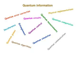
Outline • Spin-Systems and NMR • Measurements • Extracting expectation values • Extracting probabilities • Noninvasive measurements • Ancilla Assisted State-Tomography • Ancilla Assisted Process-Tomography • Quantum Simulations • Particle in a potential • Introducing quantum noise • Phase Encoding (Quantum Sensors) • Diffusion in liquids • Mapping-out electromagnetic fields • Summary
Nuclear Spin and Magnetic Resonance 1H B0 Spin ½ (qubit) 1 0 EM energy (Radio waves) Chloroform
Nuclear Spin and Magnetic Resonance B0 1 0 EM energy (Radio waves)
Nuclear Spin and Magnetic Resonance NMR Signal x Tr[ x ] x x Net transverse magnetization Procedure: Prepare t
Ancilla assisted measurement: Unitary observable 13C 1H System qubit Prepare Ancilla qubit Prepare |+ x = A x x System qubit Prepare A1 A2 Am A Ancilla qubit Prepare |+ x = A1 A2 Am O. Moussa et al, PRL,104, 160501 (2010)
Example: Evaluating Leggett-Garg inequality A. J. Leggett and A. Garg, PRL-1985 Hamiltonian : H = ½ z Johannes Kofler, PhD Thesis, 2004 13C 1H x↗ x↗ x(0)x(t) = C12 0 0 Macrorealistic: K3= C12 + C23 C13 1 For spin ½ : K3 = 2cos(t) cos(2t) (-3 K3 -1.5) x↗ x↗ x(t)x(2t) = C23 0 x(0)x(2t) = C13 x↗ x↗ t = 0 t 2t time Athalye, S. S. Roy, TSM, PRL-2011 t
Example: Evaluating Leggett-Garg inequality A. J. Leggett and A. Garg, PRL-1985 Hamiltonian : H = ½ z Johannes Kofler, PhD Thesis, 2004 13C 1H x↗ x↗ x(0)x(t) = C12 0 0 Macrorealistic: K3= C12 + C23 C13 1 For spin ½ : K3 = 2cos(t) cos(2t) (-3 K3 -1.5) x↗ x↗ x(t)x(2t) = C23 0 x(0)x(2t) = C13 x↗ x↗ t = 0 t 2t time Athalye, S. S. Roy, TSM, PRL-2011
Extracting probabilities (in computational basis) Arbitrary 1q density matrix Diagonal density matrix Single quantum density matrix crusher convert measure U incoherence (dephasing channel) x U Prepare t
Extracting joint probabilities Suppose Q be an observable, with eigenvalues q = 0 or 1 t t+t System qubit p( q(t),q(t+ t) ) ? System qubit Prepare U(t) q(t) q(t+ t) x x U(t) Ancilla qubit Prepare|0
Extracting joint probabilities: Noninvasive method (Negative Result) Suppose Q be an observable, with eigenvalues q = 0 or 1 t t+t System qubit p( q(t),q(t+ t) ) ? System qubit System qubit Prepare Prepare U(t) U(t) q(t) q(t+ t) x x x x Discord q = 1 --------------------- p(0,0) & p(0,1) U(t) U(t) Ancilla qubit Ancilla qubit Prepare|0 Prepare|0 Discord q = 0 --------------------- P(1,0) & p(1,1)
Extracting joint probabilities ancilla t1 system H C Q1 Q2 Q3 time t2 t3 p(q1,q2) p(q1,q3) Hemant, Abhishek, Koteswar, TSM,PRA-2013
A. R. Usha Devi, H. S. Karthik, Sudha, and A. K. Rajagopal, PRA-2013 Entropic Leggett-Garg Inequality ancilla System state: 1/2 system Dynamical observable : Sz(t) = UtSzUt† t1 Time Evolution: Ut = exp(iSxt) H C Information Deficit: Q1 Q2 Q3 . . . time t2 t3 . . . Hemant, Abhishek, Koteswar, TSM,PRA-2013
A. R. Usha Devi, H. S. Karthik, Sudha, and A. K. Rajagopal, PRA-2013 Reason for LGI violation: P(q2,q3) P(q1,q3) P(q1,q2) P’(q1,q2) = P(q1,q2,q3) P’(q2,q3) = P(q1,q2,q3) P’(q1,q3) = P(q1,q2,q3) Classical Probability Theory: q2 q3 q1 Marginals Grand Quantum systems do not obey this rule !!
Extracting GRAND probabilities: Suppose Q be an observable, with eigenvalues q = 0 or 1 p(q(0),q(t),,q(nt)) ? 0 t (n-1)t nt System qubit Q(0) q(t) q((n-1)t) Q(nt) Prepare U(t) U(t) U(t) U(t) System qubit x x Prepare|0 n ancilla qubits Prepare|0 Prepare|0
Illegitimate Joint Probability Hemant, Abhishek, Koteswar, TSM, PRA-2013 P(q1,q2,q3) is illegitimate !! Violation of Entropic LGI
Quantum State Tomography Tomography:
Quantum State Tomography • Complete characterization of complex density matrix • Requires a series of measurements all starting from same initial condition = + 3-unknowns Obtained by measuring z Obtained by measuring x and y Measure: x(1) |00|, x(1) |11|, |00| x(2), |11| x(2), Complex signal of Two-qubits 9 different experiments carried out After rotations: II, XI, YI, IX, IY, XX, XY, YX, YY 15-unknowns
Quantum State Tomography: Scaling Number unknowns in the density matrix n-qubit system: 22n 2n Number of experiments ~ = n 2n n Observables per experiment number of experiments 19 11 7 4 3 2 2 n-qubits 2n x 2n density matrix
Ancilla Assisted Quantum State Tomography: Nieuwenhuizen & coworkers, PRL-2004 Ucomp System qubits System qubits |00…0 System qubits Utomo ancillaqubits ancillaqubits |00…0 ancillaqubits x Number unknowns in the density matrix (n+a)-qubit system: 22n 2n - a Number of experiments ~ = n 2(n+a) n Observables per experiment
Ancilla Assisted Quantum State Tomography: Scaling 2n - a n (n) (a) Abhishek, Koteswar, TSM, PRA-2013
Ancilla Assisted Quantum State Tomography: 3-system qubits, 2-ancilla qubits Fidelity: 0.95 Abhishek, Koteswar, TSM, PRA-2013
Ancilla Assisted Quantum State Tomography: Noisy Measurements Abhishek, Koteswar, TSM, PRA-2013
Quantum Process Tomography: - Characterizes the process (unitary or nonunitary) () = mnEmEn† Standard method: mn 1 tomo b1 matrix 1 tomo b2 tomo b3 1 tomo b4 1
Ancilla Assisted Process Tomography: Altepeter et al, PRL-2003 - Characterizes the process (unitary or nonunitary) () = mnEmEn† Using a single ancillaqubit mn matrix (on system) 1 1 tomo 1 1
Single-Shot Process Tomography: - Characterizes the process (unitary or nonunitary) () = mnEmEn† Using two ancillaqubits mn matrix x process (on system) 1 1 1 1
Quantum Simulation: Particle in a potential (1D) Schrodinger equation: iħ (d/dt) |(t) = H|(0) |(t) = exp(-iHt)|(0) H = T + V Potential Kinetic P2/2m Do not commute Trotter approximation: exp(-i H dt) exp(-i V/2 dt) . exp(-i T dt) . exp(-i V/2 dt)
Quantum Simulation: Particle in a potential (1D) (with spin-1/2 nuclei) x position |111 |110 |101 |100 |011 |010 |001 |000 Trotter form: exp(-i H dt) exp(-i V/2 dt) . exp(-i T dt) . exp(-i V/2 dt) exp(-i H dt) exp(-i V/2 dt) .Uiqft. exp(-i T’ dt) . Uqft. exp(-i V/2 dt) Circuit for Diagonal Unitary
AncillaAssited Quantum Simulation: Initial state Final state (after Simulation) Ravi Shankar, SwathiHegde, TSM, PLA-2013
AncillaAssited Quantum Simulation: Ravi Shankar, SwathiHegde, TSM, PLA-2013 Experiments Theory
Simulating quantum noise: Cory & coworkers PRA, 2003 1H (system) 13C (ancilla: environment) chloroform System System Time Time Ancilla Ancilla kicks
Simulating quantum noise: 1H (system) 13C (environment) chloroform Has applications in optimizing dynamical decoupling sequences Swathi & TSM (on-going work)
Measuring diffusion |0+|1 |0+ei|1 B0 Price, Concepts in NMR-1997
Measuring diffusion |0+|1 |0+ei|1 B0 Price, Concepts in NMR-1997
Measuring diffusion 31P Trimethylphosphite (300 K, DMSO, fixed conc.) Abhishek, Manvendra, TSM, CPL-2013
Measuring diffusion: NOON states |0…0+|1…1 |0…0+ein|1…1 B0 31P 10-qubits Converting to single-quantum states Preparing NOON states Trimethylphosphite (300 K, DMSO, fixed conc.) Abhishek, Manvendra, TSM, CPL-2013
Measuring diffusion: NOON states 31P Trimethylphosphite (300 K, DMSO, fixed conc.) Abhishek, Manvendra, TSM, CPL-2013
Mapping RF Intensity with NOON states: 31P Abhishek, Manvendra, TSM, CPL-2013
Summary: • Ancillaqubits play an important role in practical quantum processors • Provide efficient ways to measure expectation values and joint probabilities • Assist in Quantum State Tomography and Quantum Process Tomography • Assist in direct read-out of probabilities in quantum simulation • Can induce controlled quantum noise on the system qubits • Can participate in preparing large NOON states – have applications in quantum sensors