Download
1 / 56
570 likes | 620 Vues
Learn about RF linear accelerators, their history, design principles, and functioning. Delve into cavity design, beam dynamics, and electromagnetic field control. Explore key concepts and developments in the field to gain a comprehensive understanding.

E N D
RF LINACS Alessandra Lombardi BE/ ABP CERN
Credits • much of the material is taken directly from Thomas Wangler USPAS course (http://uspas.fnal.gov/materials/SNS_Front-End.ppt.pdf) and Mario Weiss and Pierre Lapostolle report (Formulae and procedures useful for the design of linear accelerators, from CERN doc server) • from previous linac courses at CAS and JUAS by Erk Jensen, Nicolas Pichoff, Andrea Pisent, Maurizio Vretenar , (http://cas.web.cern.ch/cas)
Contents • PART 1 (today) : • Introduction : why? ,what?, how? , when? • Building bloc I (1/2) : Radio Frequency cavity • From an RF cavity to an accelerator • PART 2 (tomorrow) : • Building bloc II (2/2) : quadrupoles and solenoids • Single particle beam dynamics • Collective effects brief examples : space charge and wake fields.
What is a linac • LINear ACcelerator : single pass device that increases the energy of a charged particle by means of a (radio frequency) electric field. • Motion equation of a charged particle in an electromagnetic field
What is a linac-cont’ed Relativistic or not type of focusing type of particle : charge couples with the field, mass slows the acceleration type of RF structure
Type of particles : light or heavy (electrons/muons) Electron mass 0.511 MeV (protons and ions) Proton Mass 938.28 MeV
Electrostatic field 750 kV Cockcroft-Walton • Linac2 injector at CERN from 1978 to 1992.
When ? A short history • Acceleration by time varying electromagnetic field overcomes the limitation of static acceleration • First experiment towards an RF linac : Wideroelinac 1928 on a proposal by Ising dated 1925. A bunch of potassium ions were accelerated to 50 keV in a system of drift tubes in an evacuated glass cylinder. The available generator provided 25 keV at 1 MHz. • First realization of a linac : 1931 by Sloan and Lawrence at Berkeley laboratory • From experiment to a practical accelerator : Wideroe to Alvarez • to proceed to higher energies it was necessary to increase by order of magnitude the frequency and to enclose the drift tubes in a RF cavity (resonator) • this concept was proposed and realized by Luis Alvarez at University of California in 1955 : A 200 MHz 12 m long Drift Tube Linac accelerated protons from 4 to 32 MeV. • the realization of the first linac was made possible by the availability of high-frequency power generators developed for radar application during World War
RF power supply Wave guide Power coupler Cavity principle of an RF linac • RF power source: generator of electromagnetic wave of a specified frequency. It feeds a • Cavity : space enclosed in a metallic boundary which resonates with the frequency of the wave and tailors the field pattern to the • Beam : flux of particles that we push through the cavity when the field is maximized as to increase its • Energy.
designing an RF LINAC • cavity design : 1) control the field pattern inside the cavity; 2) minimise the ohmic losses on the walls/maximise the stored energy. • beam dynamics design : 1) control the timing between the field and the particle, 2) insure that the beam is kept in the smallest possible volume during acceleration tomorrow
electric field in a cavity • assume that the solution of the wave equation in a bounded medium can be written as • cavity design step 1 : concentrating the RF power from the generator in the area traversed by the beam in the most efficient way. i.e. tailor E(x,y,z) to our needs by choosing the appropriate cavity geometry. function of space function of time oscillating at freq = ω/2π
y x z cavity geometry and related parameters definition field beam Cavity 1-Average electric field 2-Shunt impedance 3-Quality factor 4-Filling time 5-Transit time factor 6-Effective shunt impedance L=cavity length
standing vs. traveling wave Standing Wave cavity : cavity where the forward and backward traveling wave have positive interference at any point
cavity parameters-1 • Average electric field ( E0 measured inV/m) is the space average of the electric field along the direction of propagation of the beam in a given moment in time when F(t) is maximum. • physically it gives a measure how much field is available for acceleration • it depends on the cavity shape, on the resonating mode and on the frequency
cavity parameters-2 • Shunt impedance ( Zmeasured inΩ/m) is defined as the ratio of the average electric field squared (E0 ) to the power (P) per unit length (L) dissipated on the wall surface. or for TW • Physically it is a measure of well we concentrate the RF power in the useful region . • NOTICE that it is independent of the field level and cavity length, it depends on the cavity mode and geometry. • beware definition of shunt impedance !!! some people use a factor 2 at the denominator ; some (other) people use a definition dependent on the cavity length.
cavity parameters-3 • Quality factor ( Q dimension-less) is defined as the ratio between the stored energy (U) and the power lost on the wall (P) in one RF cycle (f=frequency) • Q is a function of the geometry and of the surface resistance of the material : superconducting (niobium) : Q= 1010 normal conducting (copper) : Q=104 example at 700MHz
cavity parameters-3 • SUPERCONDUCTING Q depends on temperature : • 8*109 for 350 MHz at 4.5K • 2*1010 for 700 MHz at 2K. • NORMAL CONDUCTING Q depends on the mode : • 104 for a TM mode (Linac2=40000) • 103 for a TE mode (RFQ2=8000).
cavity parameters-4 • filling time ( τ measured in sec) has different definition on the case of traveling or standing wave. • TW : the time needed for the electromagnetic energy to fill the cavity of length L • SW : the time it takes for the field to decrease by 1/e after the cavity has been filled velocity at which the energy propagates through the cavity measure of how fast the stored energy is dissipated on the wall
cavity parameters-5 • transit time factor ( T, dimensionless) is defined as the maximum energy gain per charge of a particles traversing a cavity over the average voltage of the cavity. • Write the field as • The energy gain of a particle entering the cavity on axis at phase φ is
cavity parameters-5 • assume constant velocity through the cavity (APPROXIMATION!!) we can relate position and time via • we can write the energy gain as • and define transit time factor as T depends on the particle velocity and on the gap length. IT DOESN”T depend on the field
cavity parameters-5 • NB : Transit time factor depends on x,y (the distance from the axis in cylindrical symmetry). By default it is meant the transit ime factor on axis • Exercise!!! If Ez= E0 then L=gap lenght β=relativistic parametre λ=RF wavelenght
cavity parameter-6 if we don’t get the length right we can end up decelerating!!!
effective shunt impedance • It is more practical, for accelerator designers to define cavity parameters taking into account the effect on the beam • Effective shunt impedance ZTT measure if the structure is optimized and adapted to the velocity of the particle to be accelerated measure if the structure design is optimized
limit to the field in a cavity • normal conducting : • heating • Electric peak field on the cavity surface (sparking) • super conducting : • quenching • Magnetic peak field on the surface (in Niobium max 200mT)
Kilpatrick sparking criterion(in the frequency dependent formula) f = 1.64 E2 exp (-8.5/E) GUIDELINE nowadays : peak surface field up to 2*kilpatrick field Quality factor for normal conducting cavity is Epeak/EoT
wave equation -recap • Maxwell equation for E and B field: • In free space the electromagnetic fields are of the transverse electro magnetic,TEM, type: the electric and magnetic field vectors are to each other and to the direction of propagation. • In a bounded medium (cavity) the solution of the equation must satisfy the boundary conditions :
TE or TM modes • TE (=transverse electric) : the electric field is perpendicular to the direction of propagation. in a cylindrical cavity • TM (=transverse magnetic) : the magnetic field is perpendicular to the direction of propagation n : azimuthal, m : radial l longitudinal component n : azimuthal, m : radial l longitudinal component
TE modes dipole mode quadrupole mode used in Radio Frequency Quadrupole
TM modes TM010 mode , most commonly used accelerating mode
cavity modes • • 0-mode Zero-degree phase shift from cell to cell, so fields adjacent cells are in phase. Best example is DTL. • • π-mode 180-degree phase shift from cell to cell, so fields in adjacent cells are out of phase. Best example is multicell superconducting cavities. • • π/2 mode 90-degree phase shift from cell to cell. In practice these are biperiodic structures with two kinds of cells, accelerating cavities and coupling cavities. The CCL operates in a π/2structure mode. This is the preferred mode for very long multicell cavities, because of very good field stability.
Mode 0 also called mode 2π. For synchronicity and acceleration, particles must be in phase with the E field on axis (will be discussed more in details later). During 1 RF period, the particles travel over a distance of βλ. The cell L lentgh should be: Named from the phase difference between adjacent cells.
Selection of accelerating structures • Radio Frequency Quadrupole • Interdigital-H structure • Drift Tube Linac • Side Coupled Linac
- - + + + + - - transverse field in an RFQ alternating gradient focussing structure with period length (in half RF period the particles have travelled a length /2 )
acceleration in RFQ longitudinal modulation on the electrodes creates a longitudinal component in the TE mode
acceleration in an RFQ modulation X aperture aperture
important parameters of the RFQ Transverse field distortion due to modulation (=1 for un-modulated electrodes) limited by sparking type of particle Accelerating efficiency : fraction of the field deviated in the longitudinal direction (=0 for un-modulated electrodes) transit time factor cell length
.....and their relation focusing efficiency accelerating efficiency a=bore radius, ,=relativistic parameters, c=speed of light, f= rf frequency, I0,1=zero,first order Bessel function, k=wave number, =wavelength, m=electrode modulation, m0=rest q=charge, r= average transverse beam dimension, r0=average bore, V=vane voltage
RFQ • The resonating mode of the cavity is a focusing mode • Alternating the voltage on the electrodes produces an alternating focusing channel • A longitudinal modulation of the electrodes produces a field in the direction of propagation of the beam which bunches and accelerates the beam • Both the focusing as well as the bunching and acceleration are performed by the RF field • The RFQ is the only linear accelerator that can accept a low energy CONTINOUS beam of particles • 1970 Kapchinskij and Teplyakov propose the idea of the radiofrequency quadrupole ( I. M. Kapchinskii and V. A. Teplvakov, Prib.Tekh. Eksp. No. 2, 19 (1970))
Interdigital H structure TE110 mode • stem on alternating side of the drift tube force a longitudinal field between the drift tubes • focalisation is provided by quadrupole triplets places OUTSIDE the drift tubes or OUTSIDE the tank
IH use • very good shunt impedance in the low beta region (( 0.02 to 0.08 ) and low frequency (up to 200MHz) • not for high intensity beam due to long focusing period • ideal for low beta heavy ion acceleration
Tuning plunger Drift tube Quadrupole lens Post coupler Cavity shell DTL – drift tubes
DTL : electric field Mode is TM010
DTL The DTL operates in 0 mode for protons and heavy ions in the range b=0.04-0.5 (750 keV - 150 MeV) Synchronism condition (0 mode): E z l=bl The beam is inside the “drift tubes” when the electric field is decelerating The fields of the 0-mode are such that if we eliminate the walls between cells the fields are not affected, but we have less RF currents and higher shunt impedance
RFQ vs. DTL DTL can't accept low velocity particles, there is a minimum injection energy in a DTL due to mechanical constraints
The Side Coupled Linac multi-cell Standing Wave structure in p/2 mode frequency 800 - 3000 MHz for protons (b=0.5 - 1) Rationale: high beta cells are longer advantage for high frequencies • at high f, high power (> 1 MW) klystrons available long chains (many cells) • long chains high sensitivity to perturbations operation in p/2 mode Side Coupled Structure: - from the wave point of view, p/2 mode - from the beam point of view, p mode