Download
1 / 8
80 likes | 186 Vues
Chapter 2 - Theory of fractals and b values. (a). n = 0. n = 1. n = 2. n = 3. n = 4. n = 5. (b). n = 2. n = 1. n = 3. n = 4. Figure 2.1 Simple deterministic fractals. (a) The Cantor set, D = 0.6309. The

E N D
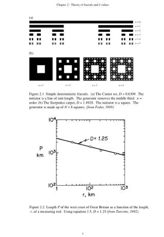
Chapter 2 - Theory of fractals and b values (a) n = 0 n = 1 n = 2 n = 3 n = 4 n = 5 (b) n = 2 n = 1 n = 3 n = 4 Figure 2.1 Simple deterministic fractals. (a) The Cantor set, D = 0.6309. The initiator is a line of unit length. The generator removes the middle third. n = order. (b) The Sierpinksi carpet, D = 1.8928. The initiator is a square. The generator is made up of N = 8 squares. (from Feder, 1989) Figure 2.2 Length P of the west coast of Great Britain as a function of the length, r, of a measuring rod. Using equation 1.5, D = 1.25 (fromTurcotte, 1992). 7
Chapter 2 - Theory of fractals and b values (b) (a) 4 10 D = 1.4 3 10 N 2 10 1 (c) (d) 10 -1 10 1 r Figure 2.3 Using the box counting method for estimating the fractal dimension of a rocky coastline. (a) is a map of the coastline of Dear Island, Maine. (b) The shaded area contains the square boxes with r = 1 km required to cover the coastline; N = 98. (c) As (b), but with 0.5 km boxes; N = 270. (d) Plot of N against r, yielding D = 1.4. (Turcotte, 1992) 10
Chapter 2 - Theory of fractals and b values Figure 2.4 Schematic diagram showing the fractal measurement method for the correlation dimension (from Xie & Pariseau, 1993). Figure 2.5 Estimation of the correlation dimension, D2, the gradient of a plot of log10C(r) against log10r. Black line represents least squares fit to points in the range rn< r < rs. 12
Chapter 2 - Theory of fractals and b values Figure 2.6 Cartoon illustrating the processes hypothesised to occur during the fracture of rocks (from Henderson & Main, 1992). 22
Chapter 2 - Theory of fractals and b values Figure 2.8 Graph showing (a) b-values and (b) fractal dimensions estimated for the Parkfield area, California. The time co-ordinate is the last earthquake in the 100-event analysis window. Large earthquakes are shown by stars (from Henderson & Main, 1992). Figure 2.9 Graph showing the correlation of b-value and fractal dimension for the Parkfield area, California. Line is fitted using the least-squares method (from Henderson & Main, 1992). 29
Chapter 2 - Theory of fractals and b values Figure 2.10 Perspective view of the seismicity, after cluster analysis, from Joâo Câmara, north-eastern Brazil. Symbols represent data points belonging to cluster 1 (circles),cluster 2 (squares), and cluster 3 (crosses). Distances on axes are in kilometers measured from an arbitrary origin (from Henderson et al., 1994). 30
Chapter 2 - Theory of fractals and b values c) Figure 2.11 Diagrams showing, for cluster 1, the evolution of (a) the b-value and (b) the fractal dimension. Error estimates are 95% confidence limits for b, and ± 10% for D. These are indicated by the vertical double-ended arrows. (c) shows the negative correlation between b and D for cluster 1 (from Henderson et al., 1994). 31
Chapter 2 - Theory of fractals and b values c) Figure 2.12 As figure 2.11, but for cluster 2 (from Henderson et al., 1994). 32